This project is a GID Problem Type (GPT) distributed under GPL V3.
I developed this project with a didactic purpose to help anyone in the engineer field to understand the basis of the Finite Element Method (FEM) and its application.
A simple physic model of steady-state heat transfer was chosen to keep the code easy to follow and legible for software engineers that are taking their first steps in Numerical Processing.
In any case, a minimum of knowledge in the involved fields are required. I will assume that you know some of Thermodynamic Principles, Differential Equations, the basis of Numerical Processing, Continuous Mechanic and stuff like that.
"GiD has been designed to cover all the common needs in the numerical simulation field from pre to post processing: geometrical modeling, effective definition of analysis data, meshing, data transfer to analysis software, as well as the visualization of numerical results."
Please refer to the next link for more details.
"When GiD is to be used for a particular type of analysis, it is necessary to predefine all the information required from the user and to define the way the final information is given to the solver module. To do so, some files are used to describe conditions, materials, general data, units systems, symbols and the format of the input file for the solver. We call Problem Type to this collection of files used to configure GiD for a particular type of analysis."
Please refer to the next link for more details.
You will find in this project:
-. The source code of the FEM implementation for the Steady-State Heat Transfer analysis in a 2D geometry. The module called CFem2DHeat was developed following Object Oriented Programming (OOP), using C++ and GNU Scientific Library (GSL).
-. The folder with all the needed files that are required for the GPT (GID Problem Type) plus the binary CFem2DHeat compiled for OSX.
-. 2 Examples of Steady-State Heat Transfer problems. One with a mix of fixed temperature and flux boundary conditions and the other with a mix of fixed temperatures and convection boundary conditions.
In this document I will explain in detail about the implementation of the CFem2DHeat Module from a Software Engineer perspective.
I will try to avoid entering in the deep universe of Physics and Geometrical Math that are involved in the FEM, but I will highly recommend to read some of the vast bibliography you can find online. This methodology can be traced back to the early 1940s, so many research and works were made in this field.
You'll see that the code has a lot of comments but I will explain a little bit more in this section about the structure and the design.
The Module is divided in three important sections:
- Pre process: Parsing the input file and initialization of the global variables.
- Numerical process: Assembling and resolving the system equation.
- Post process: Generating the output file.
These sections are clearly discernible in the main.cpp file.
The main function begin with the reading of the incoming arguments in order to identify the "input file" argv[1] and the "verbosity level" argv[2].
  string fileName = argv[1] ? (string)argv[1] + ".dat" : "";
  string verbose = argv[2] ? (string)argv[2] : "";
The input is a simple text file with a special format specified by the GPT Template file called CFem2DHeat.bas. This file is required in order to define the Problem Type.
You can find more about it in the next link section "Template File".
There is a static object called TInputParser that will extract the information from the "input file" and will initialize the global variables like the Elements, Nodes, Conditions and Materials. Everything will be stored in memory, so be aware of big files.
The TInputParser class has the TInputParser::readFile function that will call the private methods to parse each section.
As you are able to see in the example input file, sections are well defined and delimited.
In first place we read the geometry unit. This value could be from meter to millimeter any in the list ('M', 'DM', 'CM', 'MM'). The geometry unit will define the factor value used to normalize the material properties as conductivity, or the boundary conditions as the flux.
It's expected that any input in the GID application for the current problem type being set as it's labelled. So, for material properties we have conductivity (k coefficient) as W/m/C° and convectivity (h coefficient) as W/mˆ2/C°; and, for Neumann boundary condition or flux, we expect W/mˆ2.
There is no other variable that require normalization by the factor value in this GPT.
The problem dimension is determined by the number of nodes and elements in the geometry. This GPT support only triangle elements for the moment, so it will be required three nodes per element. You will see in future sections, that the integration of other kind of geometry element types, are relatively easy.
Right after the dimension section there is the materials section with a list of the materials used in the geometry. The material list will be defined as:
- One column for the material ID
- Another one for the conductivity (k coefficient)
- And the last one for the convectivity (h coefficient)
There are three kind of boundary condition that this GPT accept.
- Fixed temperature, that can be applied to nodes or lines.
- Flux that require to be applied to lines.
- And Convection that also require to be applied to lines.
For this reason the conditions section is split in four sub sections, Fixed temperature in node, Fixed temperature in line, Flux in line and Convection in line. All the sub sections are processed by the same method TInputParser::parseCondition.
If there are conditions overlapped in the same node then, if it is the same condition we apply the average of the values. If it not the same condition, then it will be overrode with the last one.
Here you will see a list of nodes identified by an ID and its respective coordinates in x and y axis.
The final section is a list of nodes connectivity. Each row represent an element and it is defined for an ID, the three nodes of the triangle and the material id.
At this point we have all the information needed to instantiate each element as TTriangle objects. The TTriangle class extend from the abstract class TElement.
The reason for this abstraction is that provide a simple way to extend the GPT compatibility to support other geometry shapes. In order to do that, you need to create a new class like TTriangle and implement the virtual methods defined in the abstract class TElement. Then add an if in the method TInputParser::parseElement to instantiate your geometry shape class instead of TElement.
All the message that the Module will print are handled by the verbosity. There are three level of verbosity. I will recommend to use the level three -vvv for didactic purpose.
If you want to improve the solver velocity in the GID application you can modify the GPT CFem2DHeat.unix.bat file to use -v instead of -vvv.
Please refer to the next link section "Executing an external program" for further information.
We need to understand first what we are modeling here. The form of the equations system for 2D linear steady state field problems can be given by the following general form of the Helmholtz equation:
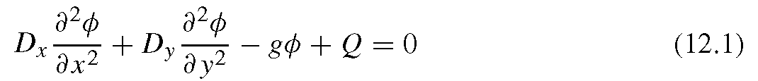
where φ is the field variable (in this case the temperature), and Dx, Dy, g and Q are given constants whose physical meaning is different for different problems (in this case Dx and Dy are the conductivity terms, g the convectivity term and Q the heat supply plus convection contribution if there is any).
I will highly recommend to read the content of the next link to understand how was the FEM implemented for this GPT.
After applying the weighted residual approach using the Galerkin method for FEM, the general form of a Helmholtz equation can be summarized as follows:

After initialize the global vectors F, A and the matrix K, we go through each element in the problem to calculate the elementary vectors and the elementary matrix.
In order to do that we read the element attributes:
  // Getting some element properties
  long double conductivity  = materials[OElement->getMaterialId()].conductivity;
  long double convectivity  = materials[OElement->getMaterialId()].convectivity;
In order to get the conductivity contribution of the element, we do:
  // Getting k element conductivity contribution
  gsl_matrix *ke  = OElement->getKd(conductivity);
OElement is an instance of TTriangle and you can see in the file TTriangle the method TTriangle::getKd defined as:
/**
 * To get the ke.
 * We calculate the k element as alpha * (Bt * B)
 * where alpha is conductivity / (4 * area)
 **/
gsl_matrix * TTriangle::getKd(long double conductivity) {
    gsl_matrix *ke = gsl_matrix_alloc(3, 3); //k element convection
    gsl_blas_dgemm(CblasNoTrans, CblasNoTrans, conductivity / (4 * area), Bt, B, 0, ke);
    return ke;
}
Where the strain matrix B and its transpose Bt are used to calculate ke. At this point ke is the matrix kd from our last equation, and our Dx/y component is determined by conductivity / (4 * area).
If you want to see how B and Bt where calculated please refer to the method TTriangle::calculateB here.
If a convective boundary condition was defined for the element then we need to obtain the km matrix and add the contribution to the ke matrix.
  // Getting k element convection contribution if any
  gsl_matrix *km  = OElement->getKm(convectivity);
You will be able to see in the file TTriangle the method TTriangle::getKm defined as:
/**
 * This method return the contribution of the convection boundary condition
 * for the K matrix element. The shape of the matrix is related with the nodes
 * involved in the boundary condition.
 * So for each nodes convination we have:
 * edge == 1   edge == 2   edge == 3
 * | 2 1 0 |   | 0 0 0 |   | 2 0 1 |
 * | 1 2 0 |   | 0 2 1 |   | 0 0 0 |
 * | 0 0 0 |   | 0 1 2 |   | 1 0 2 |
 * The contribution is determined scaling the matrix km by the convectivity factor:
 * (convectivity * L) / 6.0
 * where L is the edge length
 **/
gsl_matrix * TTriangle::getKm(long double convectivity) {
    gsl_matrix *km = gsl_matrix_alloc(3, 3); //k element convection
    gsl_matrix_set_all(km, 0);
    size_t i = -1, j = -1; size_t c = 0;
    map<size_t, SCondition>::iterator it;
    for (it = conditions.begin(); it != conditions.end(); it++) {
        if (it->second.type == "Convection") {
            if (i == -1) i = c; else j = c;
        }
        c++;
    }
    if (i != -1 && j != -1) {
        size_t k = getEdgeIndex(i, j);

        if (k == 0) {
            gsl_matrix_set(km, 0, 0, 2); gsl_matrix_set(km, 0, 1, 1); gsl_matrix_set(km, 0, 2, 0);
            gsl_matrix_set(km, 1, 0, 1); gsl_matrix_set(km, 1, 1, 2); gsl_matrix_set(km, 1, 2, 0);
            gsl_matrix_set(km, 2, 0, 0); gsl_matrix_set(km, 2, 1, 0); gsl_matrix_set(km, 2, 2, 0);
        }

        if (k == 1) {
            gsl_matrix_set(km, 0, 0, 0); gsl_matrix_set(km, 0, 1, 0); gsl_matrix_set(km, 0, 2, 0);
            gsl_matrix_set(km, 1, 0, 0); gsl_matrix_set(km, 1, 1, 2); gsl_matrix_set(km, 1, 2, 1);
            gsl_matrix_set(km, 2, 0, 0); gsl_matrix_set(km, 2, 1, 1); gsl_matrix_set(km, 2, 2, 2);
        }

        if (k == 2) {
            gsl_matrix_set(km, 0, 0, 2); gsl_matrix_set(km, 0, 1, 0); gsl_matrix_set(km, 0, 2, 1);
            gsl_matrix_set(km, 1, 0, 0); gsl_matrix_set(km, 1, 1, 0); gsl_matrix_set(km, 1, 2, 0);
            gsl_matrix_set(km, 2, 0, 1); gsl_matrix_set(km, 2, 1, 0); gsl_matrix_set(km, 2, 2, 2);
        }

        gsl_matrix_scale(km, (convectivity * getEdgeLength(k)) / 6.0);
    }

    return km;
}
This method seems more complex than the one before so lets give a closer look. First, we need to check if the element has a convective condition in one of its edges.
If there is not condition then no even one loop will be perform in the for (it = conditions.begin(); it != conditions.end(); it++) and of course the if (i != -1 && j != -1) will be false.
If the element has a convective condition only applying to one of its node then j == -1 and the if (i != -1 && j != -1) will be false too.
So, the only way that the method return some contribution for a convective condition will happen if at least two nodes of the element are affected for it, in which case the contribution is determined for the edge of the element conformed for the two nodes affected.
 * edge == 1   edge == 2   edge == 3
 * | 2 1 0 |   | 0 0 0 |   | 2 0 1 |
 * | 1 2 0 |   | 0 2 1 |   | 0 0 0 |
 * | 0 0 0 |   | 0 1 2 |   | 1 0 2 |
That's the reason that justify the existence of i and j and the private method TTriangle::getEdgeIndex.
Then, the convectivity contribution will be determined by one of these matrices scaled by (h * l) / 6 where h is the convection coefficient and l the length of the edge, in our case (convectivity * getEdgeLength(k)) / 6.0.
Going back to the main file, after obtain the kd and km matrices, we need to calculate the fe.
// Getting element boundary condition contributions
  gsl_vector *fe  = OElement->getF(); // f element contribution (Fix temperature if any)
  gsl_vector *fec = OElement->getFConvection(convectivity); // f element convection contribution
  gsl_vector *fef = OElement->getFFlux(convectivity); // f element flux contribution
The method TTriangle::getF is trivial so lets focus in the other two. TTriangle::getFConvection and TTriangle::getFFlux are very similar and they follow more or less the same pattern than the TTriangle::getKm function.
First we look for at least two nodes affected by the condition in order to obtain the vector contribution.
 * edge == 1   edge == 2   edge == 3
 * | 1 |       | 0 |       | 1 |
 * | 1 |       | 1 |       | 0 |
 * | 0 |       | 1 |       | 1 |
Then we scale the vector for the alpha that apply.
For TTriangle::getFConvection, alpha is (h * Ta * l) / 2 in our case convectivity * it->second.ambient * getEdgeLength(getEdgeIndex(i, j)) / 2.
For TTriangle::getFFlux, alpha is (flux * l) / 2 in our case it->second.flux * getEdgeLength(getEdgeIndex(i, j)) / 2.
As another section inside the element loop we have the assembling. In this section we do another loop for each node in the element. In this way, I get the position of the node in the global variables K and F.
It is a very simple algorithm easy to follow. It goes through each value in our elementary matrix ke and add it to the global matrix K in the proper row and column position. Similar with our elementary vectors fe, fec and fef.
At the end of this loop we will have our global matrix K and the global vector F populated with all the data needed for our lineal equation system.
The next step is to solve it and for that I use the House Holder method from the GSL.
  /**
   * Solving linear K/F equation using House Holder solver
   **/
  gsl_linalg_HH_solve(K, F, A);
And that's it... we have the temperature distribution in our vector A.
Note: For the moment I developed a really poor estimation of the flux vectors and for that, the improvement of this section is in the TODO list with high priority, for this reason I will not spend time to explain something that I hope I will change soon.
The most simple but not less important section of our module is the post process, where we store in a text file with a special format the results we get. The format of the file is determined by GID and you can read more about it here.
You can see an example of the output in the file test_flux.post.res.
Do not forget that the binary file in the GPT folder is compiled for OSX.
If you add the GPT folder into the GID Problem type folder for a different OS, then you need to re build the module and generate the proper binary file for your OS.
- Really poor gradient estimation from temperature distribution. Research and implement a better approach of flux estimation. For example "Super convergent points for the flux".
- Define a procedure and create a document for anyone that want to contribute to the project.