Written by Michele Wiseman
iNaturalist is a wonderful tool that helps bridge the gap between citizen scientists and research scientists. When iNaturalist observers take high quality photographs of taxa, upload them with geodata, and include relevant notes, these data can then be used in a multitude of studies such examining biodiversity, monitoring endangered species, understanding species hybridization, tracking invasive species, etc.
The more CS you are exposed to, the more patterns you’ll recognize in well designed databases and websites. iNaturalist is no different. Let’s look at OSU’s mascot, the American beaver, as an example.
Reference the url and you’ll notice that the beaver is given a taxon ID: 43794. This is true for all taxa on iNaturalist. Further, you can actually specify a location in the url (the default is “any”). When you realize this, you can actually hack the iNaturalist search system by appending the urls to search for multiple taxa and specific locations. For example, let’s look for the American beaver and the the common, pitiful, mallard (just kidding, just kidding, I’m not speciest here).
But really… who’s the keystone species here?
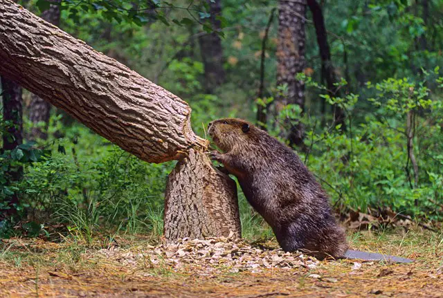
Anyway, first, let’s search for the American beaver (Castor canadensis):
https://www.inaturalist.org/observations?place_id=any&taxon_id=43794
Now, let’s search for the common mallard (Anas platyrhynchos):
https://www.inaturalist.org/observations?place_id=any&taxon_id=6930
Now, let’s combine those by using the taxa IDs for each species
https://www.inaturalist.org/observations?place_id=any&taxon_ids=6930,43794
Note the small changes: from taxon_id to taxon_ids and by adding a
common between the two numerical taxa IDs. Notice also that Anas
platyrhynchos also includes Anas platyrhynchos domesticus… why can’t
ducks just be simple? Let’s exclude the domestic mallard using a little
url hack. First, determine the taxa ID (by searching) for the domestic
mallard: 236935.
Then, let’s exclude it by adding a layer to our url using
&without_taxon_id=
https://www.inaturalist.org/observations?place_id=any&taxon_ids=6930,43794&without_taxon_id=236935
Ah, yes, clean data. I don’t believe you can combine distantly related organisms like this using their GUI search bar.
What about location? This one is a little trickier because you need to figure out the code for a given location. Locations can vary greatly in size (ex. city vs. country) so coming up with a numerical code for all these combinations isn’t intuitive. Fortunately, iNaturalist already has a bunch of codes mapped out, so we can start with those and build our own bounding boxes if necessary.
Let’s learn more about the charismatic Witch’s Hat fungus (Hygrocybe conica). I’m curious if it occurs in Oregon, so let’s specify the location as Oregon.
Note the URL change:
https://www.inaturalist.org/observations?place_id=10&taxon_id=51872
That means the ID for Oregon as a location is 10. Gosh, I always knew
Oregon was in the top 10 locations worldwide 😄. Alas, there are 19
observations in Oregon! So exciting!
Anyway, you can rinse an repeat to get an idea for what a location’s
place_id is. If you need a highly specific bounding box (ex: the
pacific northwest united states), then you can determine the coordinate
limits of the bounding box and specify them in your url. There’s a nice
tool that helps with bounding box determination
here, you can use google
maps, or you can create a bounding box in iNaturalist by clicking
Redo search in map. You’ll notice the url will change to include a
bounding box.
https://www.inaturalist.org/observations?nelat=46.10247185289826&nelng=-108.84620793472955&place_id=any&subview=map&swlat=41.75359135029721&swlng=-129.19288762222956&taxon_id=51872
More URL hacks here.
The last important thing to mention about iNaturalist is that the data available vary greatly in quality. Because neither you nor I can know the taxonomic details of all species, we are relying on trusted identifiers (i.e. scientists) to manually curate poor quality observations and a very complicated (and flawed) machine learning algorithm that automatically identifies taxa for the observers. One way to try and improve the quality of your data is to only include “Research Grade” identifications. This means there’s avaible GPS coordinates and that there has been agreement amongst a minimum of 2/3s identifiers for any given observation. You do not need any qualifications to provide input on taxonomic IDs, so sometimes the blind lead the blind and, therefore, even research grade observations should be taken with skepticism.
One way to quickly utilize these data is to use the R package rinat to
mine iNaturalists’ public database for taxa, locations, observations,
etc. of particular interest to you. For full documentation of rinat
download their pdf:
here (or you
can always load the package and get help with particular commands using
?commandhere).
#only install them if necessary, if not delete the install commands or comment them out using a hashtag
#install.packages("tidyverse")
#install.packages("rinat")
#install.packages("maps")       #only for mapping with iNat in R.

#next you need to tell R to load the packages you just installed. You need to do this every time you open R.
library(tidyverse)
library(rinat)
library(maps)R is open source and therefore has packages that are notoriously outdated, error-prone, etc. You can always check the status of a package by looking at its cran repository information. The cran page for a package will tell you when it was last updated, any necessary dependencies for the package, will link you to the reference manual, and will link you to a page where you can submit bug fix requests. Most packages are on cran.
rinat is very intuitive as long as you know how to obtain the taxon
id, place id, and what observation grade means. Let’s look at the
pacific golden chanterelle as an example (gives us a head start to
mushroom hunting season).
#use rinat package to download a inat dataframe

chanterelle_inat_oregon <- get_inat_obs(
  taxon_id = 120443,
  place_id = 10,                  #This is for Oregon
  quality = "research",
  geo = TRUE,                     #Specifies that we want geocoordinates
  maxresults = 1000,              #Limits results... too many and it'll be cumbersome to work with locally
  meta = FALSE
)

#View(chanterelle_inat_oregon)    #uncomment to preview your dataframe
You can then choose to directly map the observations using their
internal mapping feature (inat_map), use it as a layer in ggplot, or
export the spreadsheet to Tableau.
Our first example is mapping with inat_map. You can figure out the different map names by looking into the map package documentation.
chanterelle_map <- inat_map(chanterelle_inat_oregon, plot = TRUE, map = "usa")

Unfortunately, customization options are pretty limited with
(inat_map), but it’s nice for quick plotting. For superior mapping,
we’d want to use ggplot2.
There’s an entire book about ggplot2, but, you can learn the package fairly quickly by understanding how ggplot2 works. In general, ggplot works using the by layering geoms, geometric objects, and then specifying the aesthetics (aes) for these geoms.
There’s a ton of customizability with ggplot, so knowing the components of a plot helps you know what you can customize.
The components of a plot are:
- a default dataset and default set of mappings for variables to aesthetics
- one or more layers each with
- a geometric object
- a statistical transformation
- a position adjustment
- a dataset
- a set of aesthetic mappings
- one scale for each aesthetic mapping
- a coordinate system
- a facet specification
For more info, check out this cheatsheet on ggplot2.
Back to the scheduled content…
#So, if we wanted to make our points a polygon and instead use ggplot, we'd change plot to FALSE. We'd also need to create a custom polygon of the map shape.

#use the map packages to make a dataframe of the polygons in map_data("state")
states <- map_data("state")

#View(states)     #uncomment to preview your dataframe

#Now we want to filter out a polygon from our states dataframe for Oregon

oregon <- states %>%
  filter(region %in% ("oregon"))    #can change to any state, just make sure to use lowercase.

#View(oregon)     #uncomment to preview your dataframe
Now lets map our iNat data to our custom Oregon polygon using ggplot. Essentially, we’ll be layering a scatterplot (the observation data) onto a custom polygon (the map of Oregon).
chanterelle_ggplot <-
  ggplot(data = oregon) +
  geom_polygon(aes(x = long,              #base map
                   y = lat,
                   group = group),
               fill = "white",            #background color
               color = "darkgray") +      #border color
  coord_quickmap() +
  geom_point(data = chanterelle_inat_oregon,               #these are the research grade observation points
             mapping = aes(
               x = longitude,
               y = latitude,
               fill = scientific_name),                    #changes color of point based on scientific name
             color = "black",                              #outline of point
             shape= 21,                                    #this is a circle that can be filled
             alpha= 0.7) +                                 #alpha sets transparency (0-1)
theme_bw() +                                               #just a baseline theme
  theme(
    plot.background= element_blank(),                      #removes plot background
    panel.background = element_rect(fill = "white"),       #sets panel background to white
    panel.grid.major = element_blank(),                    #removes x/y major gridlines
    panel.grid.minor = element_blank())                    #removes x/y minor gridlines

chanterelle_ggplot                                         #this allows you to see the map
If we wanted to customize the labels on our chart, we can do that by
adding another layer to our chanterelle_ggplot dataframe using
labs().
chanterelle_ggplot +
  labs(title = "Pacific Golden Chanterelle iNaturalist Observations in Oregon")
It’s probably obvious that we’re plotting geodata, so I often like to
omit the x/y axis labels on maps. You can do this by defining x/y labs
as empty in theme() using
axis.title = element_blank(). There’s so much theme customization you
can do. Check out
here for more
modifications under theme().
chanterelle_ggplot +
  labs(title = "Pacific Golden Chanterelle iNaturalist Observations in Oregon") +
  theme(
    axis.title = element_blank()
  )
Lastly, lets fix the legend. Scientific names are always italicized…
plus that title is ugly (and unnecessary with only one species). We can
change the legend name by setting
theme(legend.title = element_blank()) and italicize our scientific
name using under theme(legend.text = element_text(face = "italic")).
chanterelle_ggplot +
  labs(title = "Pacific Golden Chanterelle iNaturalist Observations in Oregon") +
  theme(
    axis.title = element_blank(),
    legend.title = element_blank(),
    legend.text = element_text(face = "italic"))
Obviously there’s a lot more you can do with iNaturalist data in R using ggplot, Shiny, etc. R is great for reproducibility because you can literally give your colleague the code and they can run it and produce the same result.
On the other hand, tools like Tableau are great because they’re just so much easier to use, but it’s hard to tell someone how to recreate what you did. Tableau is improving, but you’ll see that very few people in the sciences use it… it’s more of a tool in business and marketing.
To export our data for use in Tableau, we’ll use the write.csv
command. This will write to your working directory. Don’t know your
working directory? Check with getwd().
write.csv(chanterelle_inat_oregon, "chanterelle_inat_oregon.csv", row.names = FALSE)Want to move to next level awesomeness? Try automating some of this process using this script:
library(rinat)

# A function to call `get_inat_obs` iteratively for each taxon_id present in a vector
batch_get_inat_obs <- function(
  taxon_ids_vector,            #No Default, so required, a vector of taxids
  place_id = 10,               #Default to 10, Oregon
  geo = TRUE,                  #Default to TRUE
  maxresults = 1000,           #Default to 1000 results max
  meta = FALSE                 #Default to FALSE
) {

  # The dataframe (empty now) which we will return at the end, once it's full of results
  return_df = data.frame()

  # Iterate over the taxon ids in `taxon_ids_vector`, querying each again inaturalist
  for (tid in taxon_ids_vector) {

    #Report status to console
    print(paste("Querying the following taxon id now:", tid))

    #Query inat here, using this taxon_id (`tid`, this iteration), and the other argument values
    #from the function declaration
    this_query = get_inat_obs(taxon_id = tid,
                              place_id = place_id,
                              geo = geo,
                              maxresults = maxresults,
                              meta = meta)

    #Add the result of `get_inat_obs` on this iteration to a growing dataframe
    return_df = rbind(return_df, this_query)
  }

  #After the loop is done, return the full dataframe
  return(return_df)
}

# The vector of taxon_ids
tids = c(47348, 48701, 415504, 63020, 48422, 49160)

# Call the function and assign the result to `oregon_edibles`
oregon_edibles = batch_get_inat_obs(tids)