Femlib
Library for Finite Element Method
Note: This page is under construction

Table of Contents [[TOC]]
This document defines functionality and interface of FemLib in OGS6. Primary role of the library is to provide users means to discretize mathematical equations (integral equations) via the theory of FEM. To make it general, the library must be related with only mathematical entities and not depend on any specific physical problems.
FemLib in OGS5 already provides adequate functionality required for FEM. Main changes of the library in OGS6 are focused on the code structure for improving its extendibility as below
- Modularization of FemLib
- Be independent from particular physics
- FE class does not include local assembly. Instead, local assembly calls FE class.
- FE class as composition
- Be flexible for extension
- Components are shape function, integration method, extrapolation method, mapping, etc.
As today’s FEM theory has various kinds of its deviations, we define the scopes of this library as below:
- The library provides discretization tools based on the classical Galerkin FEM with C0 elements. C1 elements are currently not supported. Discretization tools mean functions for interpolation, extrapolation and integration.
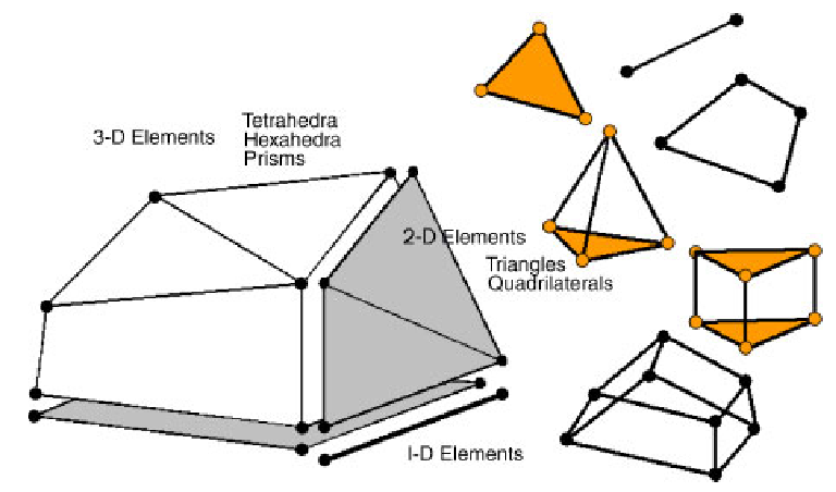
- The library supports multi-dimensional elements (1-3D). Supported shapes are line, quad, triangle, hex, tetrahedral, pyramid and prismatic. Axisymmetric and mixed-dimension problems are also supported.
- TODO: Adaptive meshing
- The library does not include other kinds of numerical methods such as time stepping method, nonlinear solution method.
- Providing basis functions for approximating continuous or discontinuous variable distributions with discrete values.
- Exmaple:

- compute basis and derivatives of basis functions for given mesh elements
- For isoparametric elements, this includes calculation of Jacobian matrix (and its inverse and determinat) for mapping from physical coordinates to natural coordinates.
- For lower-dimensional elements, this includes calculation of local coordinates from global coordinates. If the elements are also isoparametric, the mapping to natural coordinates has to be done after getting the local coordinates.
- Exmaple:
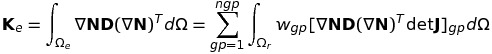
- Numerical integration over a mesh element ant along its part of boundary for, e.g. local assembly and calculation of Neumann conditions.
- Examples
- Volume integration of a Laplace term:
- Boundary integration of a Neumann condition:

- Volume integration of a Laplace term:
- Analytical integration is available only for limited cases, e.g. linear triangle elements with constant parameters.
- Numerical integration is normally used to evaluate any integrand over arbitrary elements. The most famous method is Gauss quadrature rule (wikipedia).
- Examples
- Conversion of one kind of discrete values to another kind, i.e. interpolation or extrapolation.
- Examples
- Interpolation of nodal temperature to temperature at integration points
- Extrapolation of flow velocity at integration points to that at nodes
- Examples
TODO:
- Integrating the Laplace term over an Isoparametric element using Gauss quadrature
if needed, map global coordinates of element nodes to local coordinates
initialize a Laplace matrix (K) with zero
for each Gauss point (gp)
   get integration point coordinates (x_gp), weighting factor (w_gp) for the given gp
   evaluate a matrix of derivatives of a shape function (dNr) at x_gp
   compute a Jacobian matrix (J) from dNr and local node coordinates
   compute invJ, detJ
   compute a matrix of derivatives of a shape function according to physical coordinates (dNx) using dNr and invJ
   evaluate a material parameter matrix D at gp
   compute K += dNx*D*dNx^T*w_gp*detJ
end for
- Interpolating value at Gauss integration points from nodal values
a vector of nodal values (nodU) are already calculated
for each Gauss point (gp)
   get integration point coordinates (x_gp) for the given gp
   evaluate a shape function vector (N) at x_gp
   compute gpU = N^T*nodU
end for
- Evaluating a spatially distributed material property at integration points in an Isoparametric element
for each Gauss point (gp)
   get integration point coordinates (x_gp) for the given gp
   evaluate a shape function vector (N) at x_gp
   map x_gp to physical coordinates X_gp
   evaluate a spatially distributed material property at X_gp
end for
- Users do not explicitly write equations for axisymmetric case. This is handled internally in FemLib.
| # | Type | Dim. | Mesh element | Nr. of DoFs | Order | Continuity | Mapping | Integration | Extrapolation |
|---|---|---|---|---|---|---|---|---|---|
| LINE2 | 1 | Line2 | 2 | 1 | C0 | Isoparametric | Gauss(ngp=2) | Linear | |
| >1 | Isoparametric & Local coord. | ||||||||
| Axis | Isoparametric & Cylinder coord. | ||||||||
| LINE3 | 1 | Line3 | 3 | 2 | C0 | Isoparametric | Gauss(2) | Linear | |
| >1 | Isoparametric & Local coord. | ||||||||
| Axis | Isoparametric & Cylinder coord. | ||||||||
| TRI3 | 2 | Tri3 | 3 | 1 | C0 | Isoparametric | Gauss(3) | Linear | |
| >2 | Isoparametric & Local coord. | ||||||||
| Axis | Isoparametric & Cylinder coord. | ||||||||
| TRI3CONST | 2 | Tri3 | 3 | 1 | C0 | - | Analytical | ||
| TRI6 | 2 | Tri6 | 6 | 2 | C0 | Isoparametric | Gauss(3) | Linear | |
| >2 | Isoparametric & Local coord. | ||||||||
| Axis | Isoparametric & Cylinder coord. | ||||||||
| QUAD4 | 2 | Quad4 | 4 | 1 | C0 | Isoparametric | Gauss | Linear | |
| >2 | Isoparametric & Local coord. | ||||||||
| Axis | Isoparametric & Cylinder coord. | ||||||||
| QUAD8 | 2 | Quad8 | 8 | 2 | C0 | Isoparametric | Gauss | Linear | |
| >2 | Isoparametric & Local coord. | ||||||||
| Axis | Isoparametric & Cylinder coord. | ||||||||
| QUAD9 | 2 | Quad9 | 9 | 2 | C0 | Isoparametric | Gauss | Linear | |
| >2 | Isoparametric & Local coord. | ||||||||
| Axis | Isoparametric & Cylinder coord. | ||||||||
| HEX8 | 3 | Hex8 | 8 | 1 | C0 | Isoparametric | Gauss | Linear | |
| HEX20 | 3 | Hex20 | 20 | 2 | C0 | Isoparametric | Gauss | Linear | |
| HEX27 | 3 | Hex27 | 27 | 2 | C0 | Isoparametric | Gauss | Linear | |
| TETRA4 | 3 | Tetra4 | 4 | 1 | C0 | Isoparametric | Gauss(5) | Linear | |
| TETRA10 | 3 | Tetra10 | 10 | 2 | C0 | Isoparametric | Gauss(5) | Linear | |
| PRISM6 | 3 | Prism6 | 6 | 1 | C0 | Isoparametric | Gauss(6) | Average | |
| PRISM15 | 3 | Prism15 | 15 | 2 | C0 | Isoparametric | Gauss(6) | Average | |
| PYRAMID5 | 3 | Pyramid5 | 5 | 1 | C0 | Isoparametric | Gauss(5) | Average | |
| PYRAMID13 | 3 | Pyramid13 | 13 | 1 | C0 | Isoparametric | Gauss(8) | Average | |
| EIE_QUAD4 | 2 | Quad4 | 4 | 1 | C0 | Isoparametric & Local coord. | Gauss | ||
| EIE_QUAD6 | 2 | Quad6 | 6 | 2 | C0 | Isoparametric & Local coord. | Gauss | ||
| EIE_TRI3 | 2 | Tri3 | 3 | 1 | C0 | Isoparametric & Local coord. | Gauss | ||
| EIE_TRI5 | 2 | Tri5 | 5 | 2 | C0 | Isoparametric & Local coord. | Gauss | ||
| EIE_HEX8 | 3 | Hex8 | 8 | 1 | C0 | Isoparametric & Local coord. | Gauss | ||
| EIE_HEX16 | 3 | Hex16 | 16 | 2 | C0 | Isoparametric & Local coord. | Gauss | ||
| EIE_PRISM6 | 3 | Prism6 | 6 | 1 | C0 | Isoparametric & Local coord. | Gauss | ||
| EIE_PRISM12 | 3 | Prism12 | 12 | 2 | C0 | Isoparametric & Local coord. | Gauss | ||
| EIE_TETRA4 | 3 | Tetra4 | 4 | 1 | C0 | Isoparametric & Local coord. | Gauss | ||
| EIE_TETRA9 | 3 | Tetra9 | 9 | 2 | C0 | Isoparametric & Local coord. | Gauss | ||
| EIE_PYRAMID5 | 3 | Pyramid5 | 5 | 1 | C0 | Isoparametric & Local coord. | Gauss | ||
| EIE_PYRAMID11 | 3 | Pyramid11 | 11 | 2 | C0 | Isoparametric & Local coord. | Gauss |
- Area of a triangle element: A_e
- Parameters

- Shape functions

- Derivatives of shape functions

- Integration of Mass term

- Integration of Laplace term

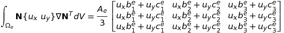
- Integration of Advection term
- Natural coordinates:

- Shape functions

- Gauss quadrature
-
Formula

-
Integration points and weights
Rule # r s w 1 point 1 1/3 1/3 1 3 points 1 1/6 1/6 1/3 2 2/3 1/6 1/3 3 1/6 2/3 1/3
-