pw_bk.Rmd

---
title: "Pathway activity inference in bulk RNA-seq"
author:
  - name: Pau Badia-i-Mompel
    affiliation:
    - Heidelberg Universiy
output: 
  BiocStyle::html_document:
    self_contained: true
    toc: true
    toc_float: true
    toc_depth: 3
    code_folding: show
package: "`r pkg_ver('decoupleR')`"
vignette: >
  %\VignetteIndexEntry{Pathway activity inference in bulk RNA-seq}
  %\VignetteEngine{knitr::rmarkdown}
  %\VignetteEncoding{UTF-8}
---

```{r setup, include=FALSE}
knitr::opts_chunk$set(
    collapse = TRUE,
    comment = "#>"
)
```
 
Bulk RNA-seq yield many molecular readouts that are hard to interpret by
themselves. One way of summarizing this information is by inferring pathway
activities from prior knowledge.

In this notebook we showcase how to use `decoupleR` for pathway activity
inference with a bulk RNA-seq data-set where the transcription factor FOXA2 was
knocked out in pancreatic cancer cell lines. 

The data consists of 3 Wild Type (WT) samples and 3 Knock Outs (KO). They are
freely available in 
[GEO](https://www.ncbi.nlm.nih.gov/geo/query/acc.cgi?acc=GSE119931).

# Loading packages
First, we need to load the relevant packages:

```{r "load packages", message = FALSE}
## We load the required packages
library(decoupleR)
library(dplyr)
library(tibble)
library(tidyr)
library(ggplot2)
library(pheatmap)
library(ggrepel)
```

# Loading the data-set
Here we used an already processed bulk RNA-seq data-set. We provide the
normalized log-transformed counts, the experimental design meta-data and the
Differential Expressed Genes (DEGs) obtained using `limma`.

For this example we use `limma` but we could have used `DeSeq2`, `edgeR` or any
other statistical framework. decoupleR requires a gene level statistic to
perform enrichment analysis but it is agnostic of how it was generated. However,
we do recommend to use statistics that include the direction of change and its
significance, for example the t-value obtained for `limma`(`t`) or `DeSeq2`(`stat`).
edgeR does not return such statistic but we can create our own by weighting the
obtained logFC by pvalue with this formula: `-log10(pvalue) * logFC`.

We can open the data like this:
```{r "load data"}
inputs_dir <- system.file("extdata", package = "decoupleR")
data <- readRDS(file.path(inputs_dir, "bk_data.rds"))
```

From `data` we can extract the mentioned information. Here we see the normalized
log-transformed counts:
```{r "counts"}
# Remove NAs and set row names
counts <- data$counts %>%
          dplyr::mutate_if(~ any(is.na(.x)), 
                           ~ dplyr::if_else(is.na(.x), 0, .x)) %>% 
          tibble::column_to_rownames(var = "gene") %>% 
          as.matrix()

head(counts)
```

The design meta-data:
```{r "design"}
design <- data$design

design
```

And the results of `limma`, of which we are interested in extracting the
obtained t-value from the contrast:
```{r "deg"}
# Extract t-values per gene
deg <- data$limma_ttop %>%
       dplyr::select(ID, t) %>% 
       dplyr::filter(!is.na(t)) %>% 
       tibble::column_to_rownames(var = "ID") %>%
       as.matrix()

head(deg)
```

# PROGENy model

[PROGENy](https://saezlab.github.io/progeny/) is a comprehensive resource containing a curated collection of pathways and their target genes, with weights for each interaction.
For this example we will use the human weights (other organisms are available) and we will use the top 500 responsive genes ranked by p-value. Here is a brief description of each pathway:

- **Androgen**: involved in the growth and development of the male reproductive organs.
- **EGFR**: regulates growth, survival, migration, apoptosis, proliferation, and differentiation in mammalian cells
- **Estrogen**: promotes the growth and development of the female reproductive organs.
- **Hypoxia**: promotes angiogenesis and metabolic reprogramming when O2 levels are low.
- **JAK-STAT**: involved in immunity, cell division, cell death, and tumor formation.
- **MAPK**: integrates external signals and promotes cell growth and proliferation.
- **NFkB**: regulates immune response, cytokine production and cell survival.
- **p53**: regulates cell cycle, apoptosis, DNA repair and tumor suppression.
- **PI3K**: promotes growth and proliferation.
- **TGFb**: involved in development, homeostasis, and repair of most tissues.
- **TNFa**: mediates haematopoiesis, immune surveillance, tumour regression and protection from infection.
- **Trail**: induces apoptosis.
- **VEGF**: mediates angiogenesis, vascular permeability, and cell migration.
- **WNT**: regulates organ morphogenesis during development and tissue repair.

To access it we can use `decoupleR`:

```{r "progeny", message=FALSE}
net <- decoupleR::get_progeny(organism = 'human', 
                              top = 500)

net
```

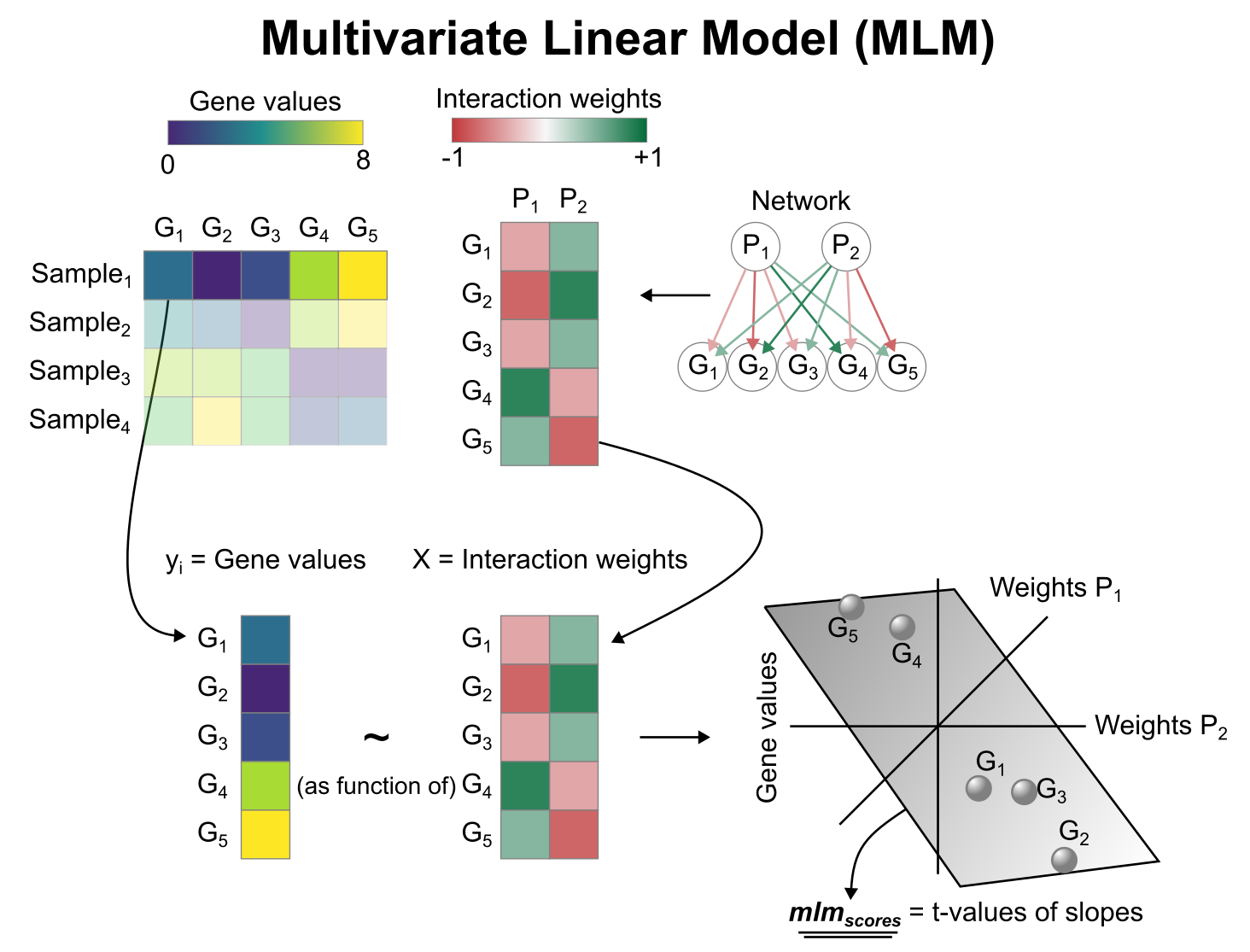
# Activity inference with Multivariate Linear Model (MLM)

To infer pathway enrichment scores we will run the Multivariate Linear Model (`mlm`) method. For each sample in our dataset (`mat`), it fits a linear model that predicts the observed gene expression based on all pathways' Pathway-Gene interactions weights.
Once fitted, the obtained t-values of the slopes are the scores. If it is positive, we interpret that the pathway is active and if it is negative we interpret that it is inactive.

![mlm](https://decoupler-py.readthedocs.io/en/1.4.0/_images/mlm.png)

To run `decoupleR` methods, we need an input matrix (`mat`), an input prior
knowledge network/resource (`net`), and the name of the columns of net that we
want to use.

```{r "sample_mlm", message=FALSE}
# Run mlm
sample_acts <- decoupleR::run_mlm(mat = counts, 
                                  net = net, 
                                  .source = 'source', 
                                  .target = 'target',
                                  .mor = 'weight', 
                                  minsize = 5)
sample_acts
```

# Visualization

From the obtained results we 
will observe the obtained activities per sample in a heat-map:
```{r "heatmap"}
# Transform to wide matrix
sample_acts_mat <- sample_acts %>%
                   tidyr::pivot_wider(id_cols = 'condition', 
                                      names_from = 'source',
                                      values_from = 'score') %>%
                   tibble::column_to_rownames('condition') %>%
                   as.matrix()

# Scale per feature
sample_acts_mat <- scale(sample_acts_mat)

# Color scale
colors <- rev(RColorBrewer::brewer.pal(n = 11, name = "RdBu"))
colors.use <- grDevices::colorRampPalette(colors = colors)(100)

my_breaks <- c(seq(-2, 0, length.out = ceiling(100 / 2) + 1),
               seq(0.05,2, length.out = floor(100 / 2)))

# Plot
pheatmap::pheatmap(mat = sample_acts_mat,
                   color = colors.use,
                   border_color = "white",
                   breaks = my_breaks,
                   cellwidth = 20,
                   cellheight = 20,
                   treeheight_row = 20,
                   treeheight_col = 20)
```

We can also infer pathway activities from the t-values of the DEGs between KO
and WT:
```{r "contrast_mlm", message=FALSE}
# Run mlm
contrast_acts <- decoupleR::run_mlm(mat  =deg, 
                                    net = net, 
                                    .source = 'source', 
                                    .target = 'target',
                                    .mor = 'weight', 
                                    minsize = 5)

contrast_acts
```

Let's show the changes
in activity between KO and WT:

```{r "barplot"}
# Plot
colors <- rev(RColorBrewer::brewer.pal(n = 11, name = "RdBu")[c(2, 10)])

p <- ggplot2::ggplot(data = contrast_acts, 
                     mapping = ggplot2::aes(x = stats::reorder(source, score), 
                                            y = score)) + 
     ggplot2::geom_bar(mapping = ggplot2::aes(fill = score),
                       color = "black",
                       stat = "identity") +
     ggplot2::scale_fill_gradient2(low = colors[1], 
                                   mid = "whitesmoke", 
                                   high = colors[2], 
                                   midpoint = 0) + 
     ggplot2::theme_minimal() +
     ggplot2::theme(axis.title = element_text(face = "bold", size = 12),
              axis.text.x = ggplot2::element_text(angle = 45, 
                                                  hjust = 1, 
                                                  size = 10, 
                                                  face = "bold"),
              axis.text.y = ggplot2::element_text(size = 10, 
                                                  face = "bold"),
              panel.grid.major = element_blank(), 
              panel.grid.minor = element_blank()) +
     ggplot2::xlab("Pathways")

p
```

The pathway p53 and Trail are deactivated in KO when
compared to WT, while MAPKK and JAK-STAT and seem to be activated.

We can further visualize the most responsive genes in each pathway along their
t-values to interpret the results. For example, let's see the genes that are 
belong to the MAPK pathway:
```{r "targets"}
pathway <- 'MAPK'

df <- net %>%
      dplyr::filter(source == pathway) %>%
      dplyr::arrange(target) %>%
      dplyr::mutate(ID = target, 
                    color = "3") %>%
      tibble::column_to_rownames('target')

inter <- sort(dplyr::intersect(rownames(deg), rownames(df)))

df <- df[inter, ]

df['t_value'] <- deg[inter, ]

df <- df %>%
      dplyr::mutate(color = dplyr::if_else(weight > 0 & t_value > 0, '1', color)) %>%
      dplyr::mutate(color = dplyr::if_else(weight > 0 & t_value < 0, '2', color)) %>%
      dplyr::mutate(color = dplyr::if_else(weight < 0 & t_value > 0, '2', color)) %>%
      dplyr::mutate(color = dplyr::if_else(weight < 0 & t_value < 0, '1', color))

colors <- rev(RColorBrewer::brewer.pal(n = 11, name = "RdBu")[c(2, 10)])

p <- ggplot2::ggplot(data = df, 
                     mapping = ggplot2::aes(x = weight, 
                                            y = t_value, 
                                            color = color)) + 
     ggplot2::geom_point(size = 2.5, 
                         color = "black") + 
     ggplot2::geom_point(size = 1.5) +
     ggplot2::scale_colour_manual(values = c(colors[2], colors[1], "grey")) +
     ggrepel::geom_label_repel(mapping = ggplot2::aes(label = ID)) + 
     ggplot2::theme_minimal() +
     ggplot2::theme(legend.position = "none") +
     ggplot2::geom_vline(xintercept = 0, linetype = 'dotted') +
     ggplot2::geom_hline(yintercept = 0, linetype = 'dotted') +
     ggplot2::ggtitle(pathway)

p
```

The pathway seems to be active since the majority of target genes with positive
weights have positive t-values (1st quadrant), and the majority of the ones with
negative weights have negative t-values (3d quadrant).

# Session information

```{r session_info, echo=FALSE}
options(width = 120)
sessioninfo::session_info()
```