tf_bk.Rmd

---
title: "Transcription factor activity inference in bulk RNA-seq"
author:
  - name: Pau Badia-i-Mompel
    affiliation:
    - Heidelberg Universiy
output: 
  BiocStyle::html_document:
    self_contained: true
    toc: true
    toc_float: true
    toc_depth: 3
    code_folding: show
package: "`r pkg_ver('decoupleR')`"
vignette: >
  %\VignetteIndexEntry{Transcription factor activity inference in bulk RNA-seq}
  %\VignetteEngine{knitr::rmarkdown}
  %\VignetteEncoding{UTF-8}
---

```{r setup, include=FALSE}
knitr::opts_chunk$set(
    collapse = TRUE,
    comment = "#>"
)
```
 
Bulk RNA-seq yield many molecular readouts that are hard to interpret by
themselves. One way of summarizing this information is by inferring
transcription factor (TF) activities from prior knowledge.

In this notebook we showcase how to use `decoupleR` for transcription factor activity
inference with a bulk RNA-seq data-set where the transcription factor FOXA2 was
knocked out in pancreatic cancer cell lines. 

The data consists of 3 Wild Type (WT) samples and 3 Knock Outs (KO). They are
freely available in 
[GEO](https://www.ncbi.nlm.nih.gov/geo/query/acc.cgi?acc=GSE119931).

# Loading packages
First, we need to load the relevant packages:

```{r "load packages", message = FALSE}
## We load the required packages
library(decoupleR)
library(dplyr)
library(tibble)
library(tidyr)
library(ggplot2)
library(pheatmap)
library(ggrepel)
```

# Loading the data-set
Here we used an already processed bulk RNA-seq data-set. We provide the
normalized log-transformed counts, the experimental design meta-data and the
Differential Expressed Genes (DEGs) obtained using `limma`.

For this example we use `limma` but we could have used `DeSeq2`, `edgeR` or any
other statistical framework. decoupleR requires a gene level statistic to
perform enrichment analysis but it is agnostic of how it was generated. However,
we do recommend to use statistics that include the direction of change and its
significance, for example the t-value obtained for `limma`(`t`) or `DeSeq2`(`stat`).
edgeR does not return such statistic but we can create our own by weighting the
obtained logFC by pvalue with this formula: `-log10(pvalue) * logFC`.

We can open the data like this:
```{r "load data"}
inputs_dir <- system.file("extdata", package = "decoupleR")
data <- readRDS(file.path(inputs_dir, "bk_data.rds"))
```

From `data` we can extract the mentioned information. Here we see the normalized
log-transformed counts:
```{r "counts"}
# Remove NAs and set row names
counts <- data$counts %>%
          dplyr::mutate_if(~ any(is.na(.x)), 
                           ~ dplyr::if_else(is.na(.x), 0, .x)) %>% 
          tibble::column_to_rownames(var = "gene") %>% 
          as.matrix()

head(counts)
```

The design meta-data:
```{r "design"}
design <- data$design

design
```

And the results of `limma`, of which we are interested in extracting the
obtained t-value and p-value from the contrast:
```{r "deg"}
# Extract t-values per gene
deg <- data$limma_ttop %>%
       dplyr::select(ID, logFC, t, P.Value) %>% 
       dplyr::filter(!is.na(t)) %>% 
       tibble::column_to_rownames(var = "ID") %>%
       as.matrix()

head(deg)
```

# CollecTRI network
[CollecTRI](https://github.com/saezlab/CollecTRI) is a comprehensive resource
containing a curated collection of TFs and their transcriptional targets
compiled from 12 different resources. This collection provides an increased
coverage of transcription factors and a superior performance in identifying
perturbed TFs compared to our previous
[DoRothEA](https://saezlab.github.io/dorothea/) network and other literature
based GRNs. Similar to DoRothEA, interactions are weighted by their mode of
regulation (activation or inhibition).

For this example we will use the human version (mouse and rat are also
available). We can use `decoupleR` to retrieve it from `OmniPath`. The argument
`split_complexes` keeps complexes or splits them into subunits, by default we
recommend to keep complexes together.

```{r "collectri"}
net <- decoupleR::get_collectri(organism = 'human', 
                                split_complexes = FALSE)

net
```

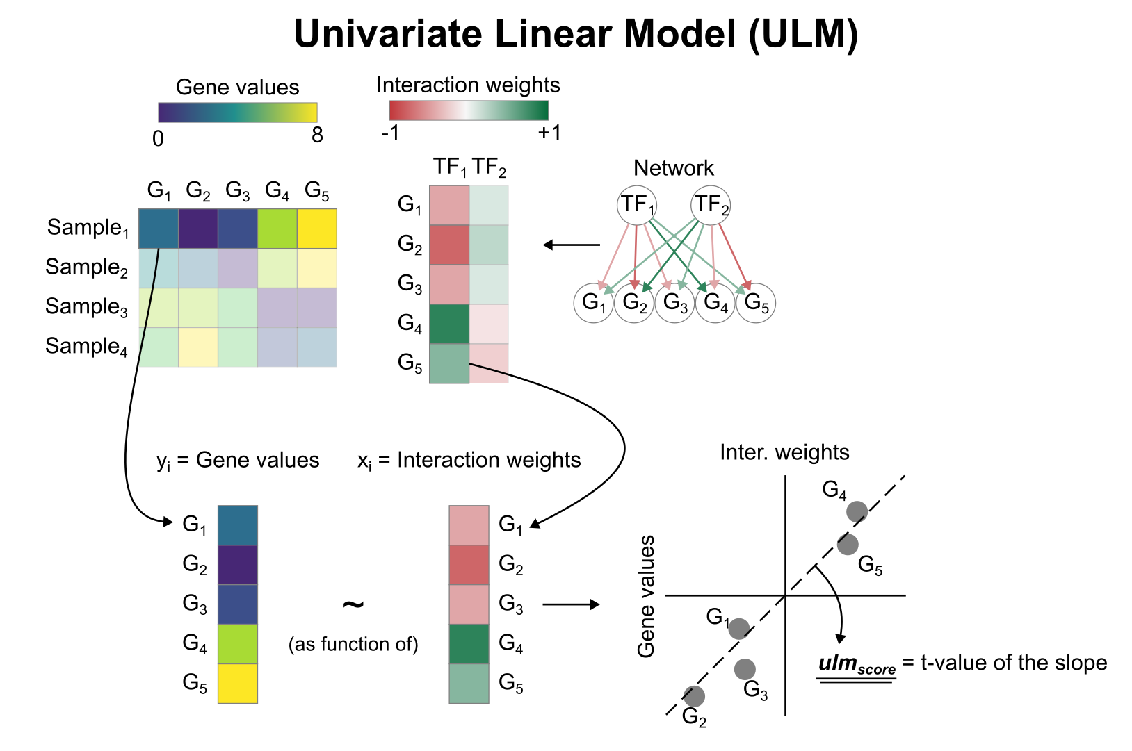
# Activity inference with Univariate Linear Model (ULM)

To infer TF enrichment scores we will run the Univariate Linear Model (`ulm`) method. For each sample in our dataset (`mat`) and each TF in our network (`net`), it fits a linear model that predicts the observed gene expression
based solely on the TF's TF-Gene interaction weights. Once fitted, the obtained t-value of the slope is the score. If it is positive, we interpret that the TF is active and if it is negative we interpret that it is inactive.

![ulm](https://decoupler-py.readthedocs.io/en/1.4.0/_images/ulm.png)

To run `decoupleR` methods, we need an input matrix (`mat`), an input prior
knowledge network/resource (`net`), and the name of the columns of net that we
want to use.

```{r "sample_ulm", message=FALSE}
# Run ulm
sample_acts <- decoupleR::run_ulm(mat = counts, 
                                  net = net, 
                                  .source = 'source', 
                                  .target = 'target',
                                  .mor = 'mor', 
                                  minsize = 5)

sample_acts
```

# Visualization

From the obtained results we will observe the most variable activities across samples in a heat-map:
```{r "heatmap"}
n_tfs <- 25

# Transform to wide matrix
sample_acts_mat <- sample_acts %>%
                   tidyr::pivot_wider(id_cols = 'condition', 
                                      names_from = 'source',
                                      values_from = 'score') %>%
                   tibble::column_to_rownames('condition') %>%
                   as.matrix()

# Get top tfs with more variable means across clusters
tfs <- sample_acts %>%
       dplyr::group_by(source) %>%
       dplyr::summarise(std = stats::sd(score)) %>%
       dplyr::arrange(-abs(std)) %>%
       head(n_tfs) %>%
       dplyr::pull(source)

sample_acts_mat <- sample_acts_mat[,tfs]

# Scale per sample
sample_acts_mat <- scale(sample_acts_mat)

# Choose color palette
colors <- rev(RColorBrewer::brewer.pal(n = 11, name = "RdBu"))
colors.use <- grDevices::colorRampPalette(colors = colors)(100)

my_breaks <- c(seq(-2, 0, length.out = ceiling(100 / 2) + 1),
               seq(0.05, 2, length.out = floor(100 / 2)))

# Plot
pheatmap::pheatmap(mat = sample_acts_mat,
                   color = colors.use,
                   border_color = "white",
                   breaks = my_breaks,
                   cellwidth = 15,
                   cellheight = 15,
                   treeheight_row = 20,
                   treeheight_col = 20)
```


We can also infer TF activities from the t-values of the DEGs between KO
and WT:
```{r "contrast_ulm", message=FALSE}
# Run ulm
contrast_acts <- decoupleR::run_ulm(mat = deg[, 't', drop = FALSE], 
                                    net = net, 
                                    .source = 'source', 
                                    .target = 'target',
                                    .mor='mor', 
                                    minsize = 5)

contrast_acts
```

Let's show the changes
in activity between KO and WT:

```{r "barplot"}

# Filter top TFs in both signs
f_contrast_acts <- contrast_acts %>%
                   dplyr::mutate(rnk = NA)

msk <- f_contrast_acts$score > 0

f_contrast_acts[msk, 'rnk'] <- rank(-f_contrast_acts[msk, 'score'])
f_contrast_acts[!msk, 'rnk'] <- rank(-abs(f_contrast_acts[!msk, 'score']))

tfs <- f_contrast_acts %>%
       dplyr::arrange(rnk) %>%
       head(n_tfs) %>%
       dplyr::pull(source)

f_contrast_acts <- f_contrast_acts %>%
                   filter(source %in% tfs)

colors <- rev(RColorBrewer::brewer.pal(n = 11, name = "RdBu")[c(2, 10)])

p <- ggplot2::ggplot(data = f_contrast_acts, 
                     mapping = ggplot2::aes(x = stats::reorder(source, score), 
                                            y = score)) + 
     ggplot2::geom_bar(mapping = ggplot2::aes(fill = score),
                       color = "black",
                       stat = "identity") +
     ggplot2::scale_fill_gradient2(low = colors[1], 
                                   mid = "whitesmoke", 
                                   high = colors[2], 
                                   midpoint = 0) + 
     ggplot2::theme_minimal() +
     ggplot2::theme(axis.title = element_text(face = "bold", size = 12),
              axis.text.x = ggplot2::element_text(angle = 45, 
                                                  hjust = 1, 
                                                  size = 10, 
                                                  face = "bold"),
              axis.text.y = ggplot2::element_text(size = 10, 
                                                  face = "bold"),
              panel.grid.major = element_blank(), 
              panel.grid.minor = element_blank()) +
     ggplot2::xlab("TFs")

p
```

The TFs GLI3 and SPDEF are deactivated in KO when
compared to WT, while MUC and NFKB1 seem to be activated.

We can further visualize the most differential target genes in each TF along their
p-values to interpret the results. For example, let's see the genes that are 
belong to SP1:
```{r "targets", warning=F}
tf <- 'SP1'

df <- net %>%
      dplyr::filter(source == tf) %>%
      dplyr::arrange(target) %>%
      dplyr::mutate(ID = target, color = "3") %>%
      tibble::column_to_rownames('target')

inter <- sort(dplyr::intersect(rownames(deg), rownames(df)))

df <- df[inter, ]

df[,c('logfc', 't_value', 'p_value')] <- deg[inter, ]

df <- df %>%
      dplyr::mutate(color = dplyr::if_else(mor > 0 & t_value > 0, '1', color)) %>%
      dplyr::mutate(color = dplyr::if_else(mor > 0 & t_value < 0, '2', color)) %>%
      dplyr::mutate(color = dplyr::if_else(mor < 0 & t_value > 0, '2', color)) %>%
      dplyr::mutate(color = dplyr::if_else(mor < 0 & t_value < 0, '1', color))

colors <- rev(RColorBrewer::brewer.pal(n = 11, name = "RdBu")[c(2, 10)])

p <- ggplot2::ggplot(data = df, 
                     mapping = ggplot2::aes(x = logfc, 
                                            y = -log10(p_value), 
                                            color = color,
                                            size = abs(mor))) + 
     ggplot2::geom_point(size = 2.5, 
                         color = "black") + 
     ggplot2::geom_point(size = 1.5) +
     ggplot2::scale_colour_manual(values = c(colors[2], colors[1], "grey")) +
     ggrepel::geom_label_repel(mapping = ggplot2::aes(label = ID,
                                                      size = 1)) + 
     ggplot2::theme_minimal() +
     ggplot2::theme(legend.position = "none") +
     ggplot2::geom_vline(xintercept = 0, linetype = 'dotted') +
     ggplot2::geom_hline(yintercept = 0, linetype = 'dotted') +
     ggplot2::ggtitle(tf)

p
```

Here blue means that the sign of multiplying the `mor` and `t-value` is negative, 
meaning that these genes are "deactivating" the TF, and red means that the sign
is positive, meaning that these genes are "activating" the TF. 

# Session information

```{r session_info, echo=FALSE}
options(width = 120)
sessioninfo::session_info()
```