梯度简单来说就是求导。 OpenCV 提供了三种不同的梯度滤波器,或者说高通滤波器:Sobel,Scharr 和 Laplacian。Sobel,Scharr 其实就是求一阶或二阶导数。Scharr 是对 Sobel(使用小的卷积核求解求解梯度角度时)的优化。Laplacian 是求二阶导数。
Sobel 算子是一个主要用作边缘检测的离散微分算子 (discrete differentiation operator)。 Sobel算子结合了高斯平滑和微分求导,用来计算图像灰度函数的近似梯度。在图像的任何一点使用此算子,将会产生对应的梯度矢量或是其法矢量。
cv2.Sobel(src,cv2.ddepth,dx,dy,Ksize)
参数意义如下:
- src:输入图像
- ddepth:输出图像的深度,支持如下src.depth()和ddepth的组合:
- 若src.depth() = CV_8U, 取ddepth =-1/CV_16S/CV_32F/CV_64F
- 若src.depth() = CV_16U/CV_16S, 取ddepth =-1/CV_32F/CV_64F
- 若src.depth() = CV_32F, 取ddepth =-1/CV_32F/CV_64F
- 若src.depth() = CV_64F, 取ddepth = -1/CV_64F
- dx:x 方向上的差分阶数
- dy:yx方向上的差分阶数
- ksize:核大小,默认值3,表示Sobel核的大小; 必须取1,3,5或7;
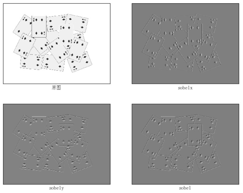
例子:sobel
def img_show(name,image):
    """matplotlib图像显示函数
    name:字符串,图像标题
    img:numpy.ndarray,图像
    """
    if len(image.shape) == 3:
        image = cv2.cvtColor(image,cv2.COLOR_BGR2RGB)
    plt.imshow(image,'gray')
    plt.xticks([])
    plt.yticks([])
    plt.xlabel(name,fontproperties='FangSong',fontsize=12)

if __name__=="__main__":
    img = cv2.imread('data/building.jpg',0)
    laplacian = cv2.Laplacian(img,cv2.CV_64F)
    #cv2.CV_64F输出图像的深度(数据类型),可以使用-1,与原图像保持一致np.uint8
    #参数1,0为只在x方向求一阶导数
    sobelx = cv2.Sobel(img,cv2.CV_64F,1,0,ksize=3)
    #参数0,1为只在y方向求一阶导数
    sobely = cv2.Sobel(img,cv2.CV_64F,0,1,ksize=3)

    #sobel =cv2.Sobel(img,cv2.CV_64F,1,1,ksize=3) # 效果不好
    sobel = cv2.add(sobelx,sobely)

    plt.figure(figsize=(10,8),dpi=80)
    plt.subplot(221)
    img_show('原图',img)
    plt.subplot(222)
    img_show('sobelx',sobelx)
    plt.subplot(223)
    img_show('sobely',sobely)
    plt.subplot(224)
    img_show('sobel',sobel)
Scharr(src, ddepth, dx, dy)
参数意义同Sobel算子
例子:scharr
def img_show(name,image):
    """matplotlib图像显示函数
    name:字符串,图像标题
    img:numpy.ndarray,图像
    """
    if len(image.shape) == 3:
        image = cv2.cvtColor(image,cv2.COLOR_BGR2RGB)
    plt.imshow(image,'gray')
    plt.xticks([])
    plt.yticks([])
    plt.xlabel(name,fontproperties='FangSong',fontsize=12)

if __name__=="__main__":
    img = cv2.imread('data/building.jpg',0)
    scharrx = cv2.Scharr(img,cv2.CV_64F,1,0)
    scharry = cv2.Scharr(img,cv2.CV_64F,0,1)

    scharr = cv2.add(scharrx,scharry)

    plt.figure(figsize=(10,8),dpi=80)
    plt.subplot(221)
    img_show('原图',img)
    plt.subplot(222)
    img_show('scharrx',scharrx)
    plt.subplot(223)
    img_show('scharry',scharry)
    plt.subplot(224)
    img_show('scharr',scharr)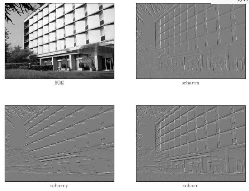
cv2.Laplacian(src,ddepth, ksize,scale,borderType)
参数意义如下:
- src:输入图像
- ddepth:输出图像的深度,支持如下src.depth()和ddepth的组合:
- 若src.depth() = CV_8U, 取ddepth =-1/CV_16S/CV_32F/CV_64F
- 若src.depth() = CV_16U/CV_16S, 取ddepth =-1/CV_32F/CV_64F
- 若src.depth() = CV_32F, 取ddepth =-1/CV_32F/CV_64F
- 若src.depth() = CV_64F, 取ddepth = -1/CV_64F
- ksize:核大小,用于计算二阶导数的滤波器的孔径尺寸,大小必须为正奇数,且有默认值1;
- scale:计算拉普拉斯值的时候可选的比例因子,有默认值1;
- borderType:默认值BORDER_DEFAUL
例子:laplacian
def img_show(name,image):
    """matplotlib图像显示函数
    name:字符串,图像标题
    img:numpy.ndarray,图像
    """
    if len(image.shape) == 3:
        image = cv2.cvtColor(image,cv2.COLOR_BGR2RGB)
    plt.imshow(image,'gray')
    plt.xticks([])
    plt.yticks([])
    plt.xlabel(name,fontproperties='FangSong',fontsize=12)

if __name__=="__main__":
    img = cv2.imread('data/building.jpg',0)
    laplacian = cv2.Laplacian(img,cv2.CV_64F,ksize=5)

    plt.figure(figsize=(10,8),dpi=80)
    plt.subplot(121)
    img_show('原图',img)

    plt.subplot(122)
    img_show('laplacian',laplacian)
在 OpenCV 中,使用函数:cv2.Canny()
cv2.Canny(image, threshold1, threshold2[, edges[, apertureSize[, L2gradient ]]])
参数解释
- image:源图像
- threshold1:阈值1
- threshold2:阈值2
- apertureSize:可选参数,Sobel算子的大小,默认值为 3
- L2gradient,它可以用来设定求梯度大小的方程。如果设为 True,就会使用方程:${E d g e_{-} \text {Gradient}(G)=\sqrt{G_{x}^{2}+G_{y}^{2}}}$,否则使用方程:${\text {Edge_Gradient}(G)=\left|G_{x}^{2}\right|+\left|G_{y}^{2}\right|}$代替,默认值为 False。
def nothing(x):
    pass
img = cv2.imread('lena.jpg')
cv2.namedWindow('edges',cv2.WINDOW_NORMAL)
cv2.createTrackbar('minVal','edges',0,255,nothing)
cv2.createTrackbar('maxVal','edges',0,255,nothing)

while(1):
    minval=cv2.getTrackbarPos('minVal','edges')
    maxval=cv2.getTrackbarPos('maxVal','edges')
    edges = cv2.Canny(img,minval,maxval)
    cv2.imshow('edges',edges)
    k=cv2.waitKey(1)&0xFF
    if k==27:
        break
cv2.destroyAllWindows()