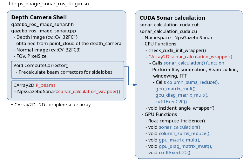
Multibeam Forward Looking Sonar
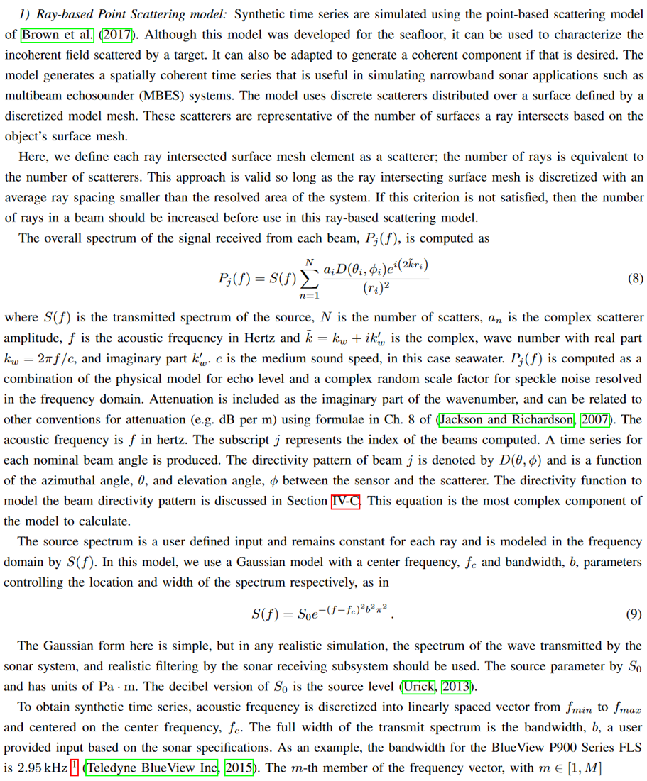
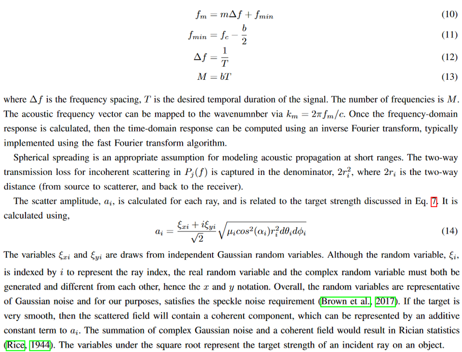
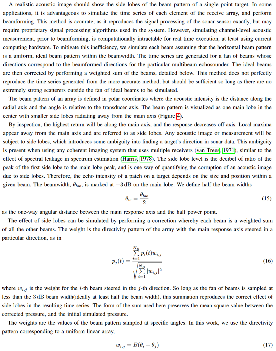
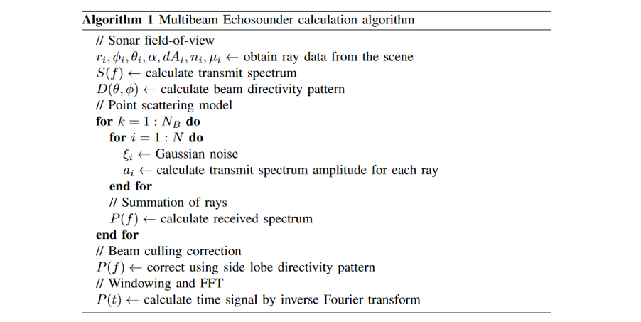
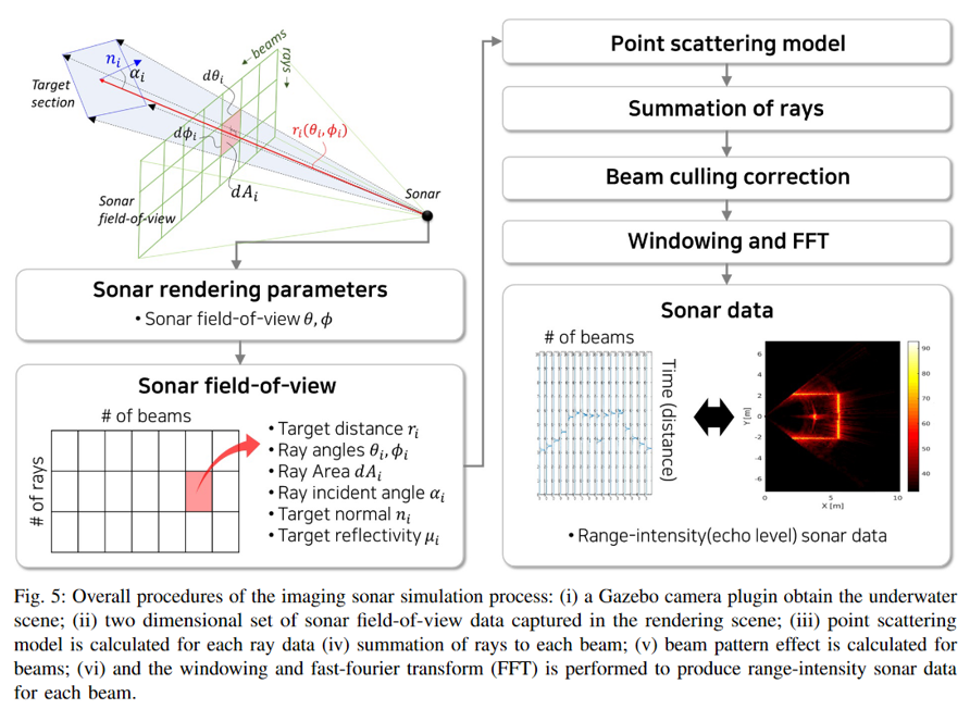
Previous sonar sensor plugins were based on image processing realms by translating each subpixel (point cloud) of the perceived image to resemble sonar sensors with or without sonar equations (Detailed Review for the previous image-based methods). Here, we have developed a ray-based multibeam sonar plugin to consider the phase and reberveration physics of the acoustic signals providing raw sonar intensity-range data (the A-plot) using the point scattering model. Physical characteristics, including time and angle ambiguities and speckle noise, are considered. The time and angle ambiguity is a function of the point spread function of the coherent imaging system (i.e., side lobes due to matched filtering and beamforming). Speckle is the granular appearance of an image due to many interfering scatterers that are smaller than the resolution limit of the imaging system.
-
Features
- Physical sonar beam/ray calculation with the point scattering model
- Generating intensity-range (A-plot) raw sonar data
- Publishes the data with UW APL's sonar image msg format
- NVIDIA CUDA core GPU parallelization
- 10Hz refresh rate with 10m range
- Physical sonar beam/ray calculation with the point scattering model
-
Original Research paper

- Note: you may need
artificialVehicleVibrationtag on to obtain sparkling sonar image
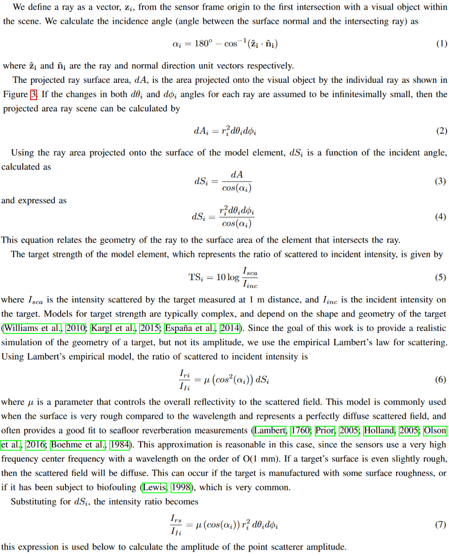
Sonar equations do not consider phase, reverberations between rays
- Source level (SL) : predefined by sonar specification
- Transmission Loss (TL) : path, absorption coefficient with ocean (temp, depth) Currently, a typical 0.0354 dB/m constant used, with a straight-line path (=distance)
- Noise Level (NL) : Ocean dependent, (maybe some statistics models exists). Currently, Gaussian noise is used.
- Directivity index (DI) : Sonar transducer specification For our purpose, having sonar resolution from the catalogue provides enough information considering typical characteristics of far-field directivity. Currently, half-power width of sinc function is used..
- Target strength (TS) : Object material, incident angle dependent. Currently, 1E-4 reflectivity constant used.
- Phase, reverberations (Implemented): For high frequency, phase overlaps and reverberations of reflected signals would be crucial, which is the case for the sonars (currently, operation frequency 900 kHz).
- Transmission paths : Transmission paths are not straight-line (=distance). The bellhop model can be discussed. This can matter in far-field searching/mission planning.
- Target strength, Surface/Bottom loss: Material, incident angle dependent target strength can be used for different objects. Obtaining correct coefficients is complicated, requiring the calculation of reflection/transmission between layers.
Work has been published describing the development of a sonar simulation model. Two of these have developed their models into supporting robotics frameworks.
In Demarco, 2015, a Gazebo sonar sensor model is developed using ray tracing. The Gazebo ray-tracing functionality generates a 3D point cloud transformed into a sonar image. On inspection, the acoustic properties were either hard-coded or commented out and did not include speckle-noise simulation.
In Cirqueira, 2017, a GPU-based sonar simulator is developed using rasterization. The model has two types of sonar: mechanically scanned imaging sonar (MSIS) and FLS. The acoustics features provided in their model are accurate and representative of sound propagation. The sonar sensor model is modelled using a virtual camera and utilizes the following three parameters to render the camera as sonar: pulse distance, echo intensity, and field-of-view. Physical tests were also conducted to compare the simulation results with the physical imaging sonar.
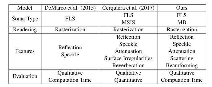
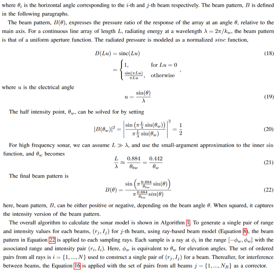
The model is based on a ray-based spatial discretization of the model facets, beampattern appropriate for a line array, and a point scattering model of the echo level.
The simplest way to prepare your machine with the CUDA library would be to use the Docker environment. Following commands include -b cuda, which provides the Cuda library.
# Uninstall rocker
sudo apt-get remove python3-rocker
sudo pip uninstall rocker

# Clone rocker fork by woensug choi
git clone [email protected]:woensug-choi/rocker.git
cd rocker

# Change to cuda-dev branch
git checkout cuda-dev

# install
sudo pip install .

# change dockwater to cuda-dev branch
cd ~/uuv_ws/src/dockwater
git checkout cuda-dev

# Build and run docker image (This may take up to 30 min to finish at the first time)
./build.bash noetic
./run.bash -c noetic:latest

# To open another terminal inside docker container,
./join.bash noetic_runtime
When docker environment is ready, clone multibeam forward-looking sonar repo and compile
# Clone necessary repos for multibeam sonar
cd ~/uuv_ws/src
vcs import --skip-existing --input dave/extras/repos/multibeam_sim.repos .

# Compile and run tutorial case
cd ~/uuv_ws
catkin build
source ~/uuv_ws/devel/setup.bash
roslaunch nps_uw_multibeam_sonar sonar_tank_blueview_p900_nps_multibeam.launchThis plugin demands high computation costs. GPU parallelization is used with the Nvidia CUDA Library. A discrete NVIDIA Graphics card is required.
- The most straightforward way to install CUDA support on Ubuntu 20 is:
sudo apt update sudo apt install nvidia-cuda-toolkit- This installs the Nvidia CUDA toolkit from the Ubuntu repository.
- If you prefer to install the latest version directly from the CUDA repository, instructions are available here: https://linuxconfig.org/how-to-install-cuda-on-ubuntu-20-04-focal-fossa-linux
Install Cuda. Install CUDA 11.1 on the host machine (Recommended installation method is to use local run file download link If you find a conflicting Nvidia driver, remove the previous driver and reinstall using a downloaded run file) This installation file will install both CUDA 11.1 and the NVIDIA graphics driver 455.32, which is best compatible with CUDA 11.1
If you have already dealt with NVIDIA graphics driver at Ubuntu Software&Updates/Additional drivers to use proprietary drivers, revert it to use 'Using X.Org X server' to avoid 'The driver already installed, remove beforehand' kind of msg when you run the installation file.
# Remove nvidia drivers
sudo apt remove nvidia-*
sudo apt autoremove
# Disable nouveau driver
sudo bash -c "echo blacklist nouveau > /etc/modprobe.d/blacklist-nvidia-nouveau.conf"
sudo bash -c "echo options nouveau modeset=0 >> /etc/modprobe.d/blacklist-nvidia-nouveau.conf"
sudo update-initramfs -u
# Reboot
sudo reboot
# Download the run file and run
# wget https://developer.download.nvidia.com/compute/cuda/11.1.1/local_installers/cuda_11.1.1_455.32.00_linux.run
sudo sh cuda_11.1.1_455.32.00_linux.run
Once you are done, you will see something like the following msg with the nvidia-smi command.
+-----------------------------------------------------------------------------+
| NVIDIA-SMI 455.32.00    Driver Version: 455.32.00    CUDA Version: 11.1     |
|-------------------------------+----------------------+----------------------+
| GPU  Name        Persistence-M| Bus-Id        Disp.A | Volatile Uncorr. ECC |
| Fan  Temp  Perf  Pwr:Usage/Cap|         Memory-Usage | GPU-Util  Compute M. |
|                               |                      |               MIG M. |
|===============================+======================+======================|
|   0  GeForce GTX 105...  Off  | 00000000:01:00.0 Off |                  N/A |
| N/A   42C    P8    N/A /  N/A |      7MiB /  4040MiB |      0%      Default |
|                               |                      |                  N/A |
+-------------------------------+----------------------+----------------------+

+-----------------------------------------------------------------------------+
| Processes:                                                                  |
|  GPU   GI   CI        PID   Type   Process name                  GPU Memory |
|        ID   ID                                                   Usage      |
|=============================================================================|
|  No running processes found                                                 |
+-----------------------------------------------------------------------------+
The final step is to add paths to the Cuda executables and libraries.
Add these lines to .bashrc to include them. You may resource it by source ~/.bshrc
export PATH=/usr/local/cuda/bin${PATH:+:${PATH}}$
export LD_LIBRARY_PATH=/usr/local/cuda/lib64${LD_LIBRARY_PATH:+:${LD_LIBRARY_PATH}}
cd ~/uuv_ws/src
vcs import --skip-existing --input dave/extras/repos/multibeam_sim.repos .
vcs will use multibeam_sim.repos file inthe dave repository that includes both nps_uw_multibeam_sonar and hydrographic_msgs.
The multibeam sonar sensor plugin is at nps_uw_multibeam_sonar repository Make sure to include the repository on the workspace before compiling.
git clone https://github.com/Field-Robotics-Lab/nps_uw_multibeam_sonar.git
Final results are exported as a SonarImage.msg of UW APL's sonar image msg format. Make sure to include the repository on the workspace before compiling.
git clone https://github.com/apl-ocean-engineering/hydrographic_msgs.git
The repository includes three sonar models (Blueview P900, Blueview M450, Seabat F50)
roslaunch nps_uw_multibeam_sonar sonar_tank_blueview_p900_nps_multibeam.launch
roslaunch nps_uw_multibeam_sonar sonar_tank_blueview_m450_nps_multibeam.launch
roslaunch nps_uw_multibeam_sonar sonar_tank_seabat_f50_nps_multibeam.launch
If you see some errors after CUDA and NVIDIA driver installation, try running catkin_make several times.
When closing the simulation with the ctrl+c command, it often hangs waiting for the Gazebo window to terminate. You can force close it using the pkill gzclient && pkill gzserver command at another terminal window.

- Note: you may need
artificialVehicleVibrationtag on to obtain sparkling sonar image
Live view capture plotted using rqt_image_view defined at Launch file

Exported data visualized with MATLAB script

The plugin outputs sonar data using the acoustic_msgs/SonarImage ROS message. This message defines the bearing of each sonar beam as a rotation around a downward-pointing axis, such that negative bearings are to port of forward and positive to starboard (if the sonar is installed in it"s "typical" forward-looking orientation).
The plugin will use the Gazebo frame name as the frame_id in the ROS message. For the sonar data to re-project correctly into 3D space, it must be attached to an X-Forward, Y-Starboard, Z-Down frame in Gazebo.
Parameters for the sonar is configured at each model.sdf file.
Viewport of the sonar is defined using depth camera parameters configuration including FOV, Clip(Range), nBeams, nRays
- Field of view (FOV)
<!-- 90 degrees for the M900-90 -->
<horizontal_fov>1.57079632679</horizontal_fov>- Range (clip)
<clip>
  <near>02</near> <!-- optimal 2m-60m -->
  <far>60</far>
</clip>- nBeams (width), nRays (height, also act as vertical field of view)
<image>
  <width>512</width>
  <!-- Set vertical FOV by setting image height -->
  <!-- Approx 2 times the spec sheet (sepc: 20 deg.) -->
  <height>224</height>
</image>- Here, the
<height>is set to define as if 40 deg, which is approximately two times that of the spec sheet. The correct vertical FOV is defined at<verticalFOV>below.
Parameters for sonar calculation are defined also at the model.sdf file including Sonar Freq, Bandwidth, Soundspeed, Source Level.
<verticalFOV>20</verticalFOV>
<sonarFreq>900e3</sonarFreq>
<bandwidth>29.9e3</bandwidth>
<soundSpeed>1500</soundSpeed>
<sourceLevel>220</sourceLevel>
<maxDistance>10</maxDistance>Calculation settings including Ray skips, Max distance, writeLog/interval, DebugFlag, Publishing topic names can be changed.
-
maxDistance: Defines max distance of the targets, which also defines the length of the signal for each beam. Ideally, it should match theclipparameter of the depth camera properties. -
ray skips: Used to reduce calculation time to jump rays to calculate. Each beam's total number of rays is defined at theheightparameter of the depth camera properties. -
sensor gain: Used to specify sensor gain for better visualization.plot scaler: Used to scale the value on the bundled viewer window, which is plotted with ROS'srqt_image_viewpackage. -
writeLogFlag : if on, raw data is saved ascsvfile at/tmp/with the rate ofwriteFrameIntervalasSonarRawData_000001.csv. You may use thescripts/plotRawData.mto plot the figures at MATLAB. -
debugFlagFlag : if on, the calculation time for each frame is printed at the console. -
artificialVehicleVibrationFlag : if on, the gaussian noise values will change constantly as sparkling sonar image in the example gif on this wiki. The sparkling noise (continuous change of random noise values even when the sonar scene is static) does not occur in the real world unless the vehicle the sonar is attached is moved or the object in the scene is changed. These physical characteristics are exploited in some scenarios to recognize the changes in the scene by detecting those noise changes. In the plugin, the Gaussian noise value (the random noise value) is changed whenever the maximum distance of the objects in the scene is changed. This flag parameter changes the random values on every frame to imitate as if the vehicle is vibrating in position.
<maxDistance>10</maxDistance>
<raySkips>10</raySkips>
<sensorGain>0.02</sensorGain>
<plotScaler>1</plotScaler>
<writeLog>false</writeLog>
<debugFlag>false</debugFlag>
<writeFrameInterval>5</writeFrameInterval>
<artificialVehicleVibration>false</artificialVehicleVibration>
<!-- This name is prepended to ROS topics -->
<cameraName>blueview_p900</cameraName>
<!-- ROS publication topics -->
<imageTopicName>image_raw</imageTopicName>
<cameraInfoTopicName>image_raw/camera_info</cameraInfoTopicName>
<pointCloudTopicName>point_cloud</pointCloudTopicName>
<depthImageTopicName>image_depth</depthImageTopicName>
<depthImageCameraInfoTopicName>image_depth/camera_info</depthImageCameraInfoTopicName>
<sonarImageRawTopicName>sonar_image_raw</sonarImageRawTopicName>
<sonarImageTopicName>sonar_image</sonarImageTopicName>
<frameName>forward_sonar_optical_link</frameName>Although high fidelity target strength is beyond reach for simple implementation, users can give different surface reflectivity on the scene's objects.
- Note
- Variational reflectivity can slow down the refresh rate significantly.
- The plugin will initiate with constant reflectivity and may take some seconds to refresh the image with variational reflectivities.
- The parameter to switch the feature is defined at
model.sdfof the sonar model (in this case,nps_uw_multibeam_sonar/models/blueview_p900_nps_multibeam/model.sdf. Assining the<constantReflectivity>and<customSDFTagReflectivity>as false will turn the variational reflectivity by the model name feature on.-
<constantReflectivity>false</constantReflectivity>
<customSDFTagReflectivity>false</customSDFTagReflectivity>
<!-- The CSV databsefile is located at the worlds folder -->
<reflectivityDatabaseFile>variationalReflectivityDatabase.csv</reflectivityDatabaseFile>
-
- Values are defined for each model object in the world. The values are defined using the CSV file in the worlds folder. The default value is 0.001. The example CSV file is at /worlds/variationalReflectivityDatabase.csv
-
basement_tank_model,0.0001
cylinder_target1,0.005
cylinder_target2,0.001
-
-
cv::Mat this->reflectivityImageis calculated if the scene is changed (it detects the change by comparing the maximum depth value of the depth camera with the previous scene. If the value is stabled (if equal for three consecutive frames, the calculation is performed once) - The
reflectivityImageOpenCV matrix is then transferred to GPU memory and used for sonar calculation

roslaunch nps_uw_multibeam_sonar sonar_tank_oculus_m1200d_nps_multibeam_customSDFTag.launch
- The parameter to switch the feature is defined at
model.sdfof the sonar model (in this case,nps_uw_multibeam_sonar/models/blueview_p900_nps_multibeam/model.sdf. Assining the<constantReflectivity>as false and<customSDFTagReflectivity>as true will turn the variational reflectivity by the custom Tag feature on. - Example tag names and how they are defined
-
<!-- Custom SDF elements for surface properties -->
<surface_props:material>metal</surface_props:material>
<surface_props:biofouling_rating>10</surface_props:biofouling_rating>
<surface_props:roughness>0.1</surface_props:roughness>
-
- You can add as many tags as you want. How they contribute to the final reflectivity is defined at the CSV file (/worlds/customSDFTagDatabase.csv)
-
biofouling_rating,20.0 roughness,5.0 default,0.001 metal,0.005 rubber,0.0001 - the material name (default, metal, and rubber) defines the base reflectivity values. The biofouling_rating, roughness, and any other tags you want to add will affect the reflectivity value as coefficients to change the base value.
-

The final output of the sonar image is sent in two types.
- Topic name
sonar_image- This is a msg used internally to plot using with
rqt_image_viewpackage of ROS. - The data is generated using OpenCV's
CV_16UC1format and changed into msg format usingMONO16format
- This is a msg used internally to plot using with
- Topic name
sonar_image_raw- This is a msg matched with UW APL's SonarImage.msg.
- The data is in
uint8.
- at workstation (i9-9900K 3.6GHz, Nvidia GeForce RTX 2080Ti)
- 10 Hz achievable with Ray and Range reduced
| 512 Beams | Refresh Rate [Hz] |
Total Time [s] |
Core | Sum | Corr | FFT |
|---|---|---|---|---|---|---|
|
Full Calculation 60 m Range 114 Rays |
0.5 Hz | 1.7 s | 0.3 | 1.26 | 0.05 | 0.03 |
|
Ray Reduced 60 m Range 11 Rays |
3.0 Hz | 0.27 s | 0.02 | 0.16 | 0.05 | 0.03 |
|
Ray/Range Reduced 10 m Range 11 Rays |
10 Hz | 0.06 s | 0.00 | 0.04 | 0.01 | 0.00 |
- Woensug Choi
- Brian Bingham
- Duane Davis
- Derek Olsen
- Bruce Allen
- Carson Vogt
- Laura Lindzey