Plotting current loops
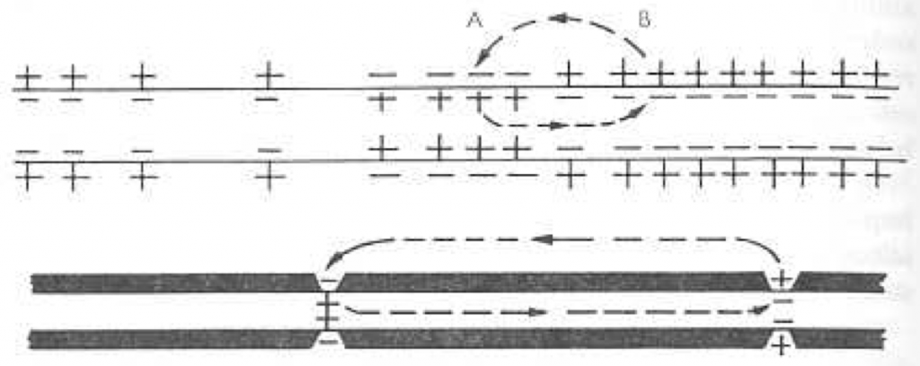
This document describes an algorithm to plot current loops in a multicompartmental simulation. « Current loop » refers to the current that enters the membrane at one point, flows intracellularly in the longitudinal dimension, goes out of the membrane, and then closes the loop extracellularly. It shows how current circulates in the neuron. Here is an example of loop shown in by Hodgkin (1964) to illustrate the spread of an action potential in an axon :
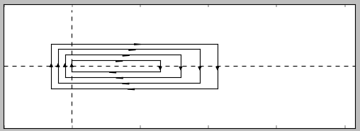
And this is the output of the current program :
First of all, I am going to restrict myself to unbranched structures, because it is not so obvious how to represent loops with branched structures. It could be for example a dendrite, soma and axon.
Basic remark
A loop is a discrete, closed object. By definition, the current should be unchanged along the loop. All loops should correspond to the same current. It follows that current loops necessarily represent a discretization of currents.
The intracellular (axial) current is I = dV/dx*(1/ra), where ra is resistance per unit length. Therefore, this can be calculated directly from the spatial profile of voltage at a given time, and the diameters of the compartments (and intracellular resistivity). The extracellular axial current is just the opposite. It seems logical to include I as a (computed) state variable in the model.
Since we need to discretize the current, a given value of current must correspond to a number of loops. For example, if the unit of current is 1 nA and the axial current is 2.3 nA, then there must be 2 current loops going to the x>0 direction (let's call that positive loop). The number of current loops at a given point is therefore : round(I) (signed). We note that a « point » corresponds to the junction between two compartments. In the following, I will then assume the substitution : I → round(I).
When the number of current loops changes, the difference must be a transmembrane current (Kirchoff's law). Let us review the different cases :
- Current goes from 2 to 3 : a new positive current loop is opened.
- Current goes from 3 to 2 : a positive current loop is closed.
- Current goes from -2 to -3 : a new negative current loop is opened.
- Current goes from -3 to -2 : a negative current loop is closed.
Thus it is important to note the same change in the number of currents has opposite meaning depending on whether currents are positive or negative. Let us consider the four border cases :
- Current goes from 0 to 1 : a new positive current loop is opened.
- Current goes from 0 to -1 : a new negative current loop is opened.
- Current goes from 1 to 0 : close
- Current goes from -1 to 0 : close
The general rule for 1-step change is therefore :
- (change*new value)>0 : open
- (change*new value)<=0 : close
where : old value = I ; new value = I' ; change = I'-I.
In case of opening, the sign of the new value determines whether a positive or negative loop is opened. In case of closure, the sign of the previous value determines whether a positive or negative loop is closed.
For a multistep change (e.g. from -2 to 3), the simplest algorithm is to iterate through all the 1-step changes.
There is an exact symetry with respect to the line y = 0. Each axial current is plotted as a horizontal segment with vertical coordinate y = +-n. Lines are joined at points where I changes. Arrows are put in the middle of segments.
Initialization can be done by applying the main iteration (next section) with I = 0 (assuming the current was previously null). Bu I am describing it separately for the sake of clarity.
I(0) determines the initial number of currents. A corresponding number of vertical lines must then be drawn. To be readable, their horizontal coordinates must be spread. The horizontal starting point of each current is stored. One question is : how to choose the vertical coordinates, given that new currents may or not open ?
One must know in advance how many current loops are going to be drawn until the next node, defined as a point of current reversal (I=0, or more precisely, I*I'<0). The algorithm is as follows :
- calculate the position of the next node (possibly the end of the neuron), defined as the next position when I changes sign ;
- calculate the max. M of abs(I) from the current position (0) to the node's position.
Then the currents must have vertical positions M-n+1 to M, and the symetrical, where n = abs(I).
We advance by one spatial step (x->x+1). If I doesn't change, we do nothing. If I changes, we iterate through 1-step changes and open or close currents as discussed above.
- closing a current : the current with the smallest y-coordinate (in absolute value) is closed, ie, a vertical line is drawn, horizontal lines are drawn from the starting point, arrows are added. This choice is necessary to avoid line crossings.
- opening a current : if currents already exist, then for the same reason, a current must be opened with vertical coordinate just below (in absolute value) the smallest one. If there are no currents (I=0), then we need to know how many currents will open in the future before the next node. We do this by applying the algorithm described in Initialization.
At the end, I might be non zero, which mean we need to close all loops. This is done by applying Iteration, with I' = 0.
- Arrow size. Dx should be proportional to the size of a compartment, or to the maximum x value (horizontal size of the plot). Dy should be proportional to the the spacing between horizontal lines, therefore a fixed value if y-coordinates are integers.
- Multiple openings/closures : x-coordinates could be spread evenly.