How MRQy works
The major components of the MRQy tool are illustrated in the Figure below, which can be sub-divided into three specific modules: Input, Backend Processing, and Front-end Visualization.

Figure 1. Schematic for overall MRQy workflow and major components.
To ensure MRQy supported popular file formats for storing radiographic data (e.g. .dcm, .nii, .mha, and .ima), the packages medpy and pydicom libraries are used. MRQy iteratively parses either a single directory input (containing files) or resources through a directory of directories, in order to read in the image volumes as well as image metadata.
As the MRI volume input to MRQy could be acquired from any body region, it is crucial to first identify the primary area within the volume from which quality measures are calculated. An in-house image processing algorithm was developed to efficiently and automatically extract and separate the background (outside the body) from the foreground (primary region of interest).
Two major types of information are extracted from each MRI volume, broadly categorized as Metadata and Measurements (summarized in the Table below). These are saved into a tab-separated file for further analysis.
-
Metadata: This information is directly extracted from file headers, such as voxel resolution or MRI volume dimensions (summarized in Rows 1-10). In addition to a default set of tags, additional metadata can be extracted from file header based on user specifications.
-
Measurements: These were selected from a survey of the medical imaging literature for detecting specific artifacts in MRI scans. This list includes statistical measures (e.g. range, variance, %CV) as well as second-order statistics and filter-based measures (e.g. contrast per pixel (CPP), entropy focus criterion (EFC), signal-to-noise ratios of different regions). Rows 13-23 summarizes the measures extracted by MRQy, their mathematical formulation, and what type of artifact they are each intended to quantify.
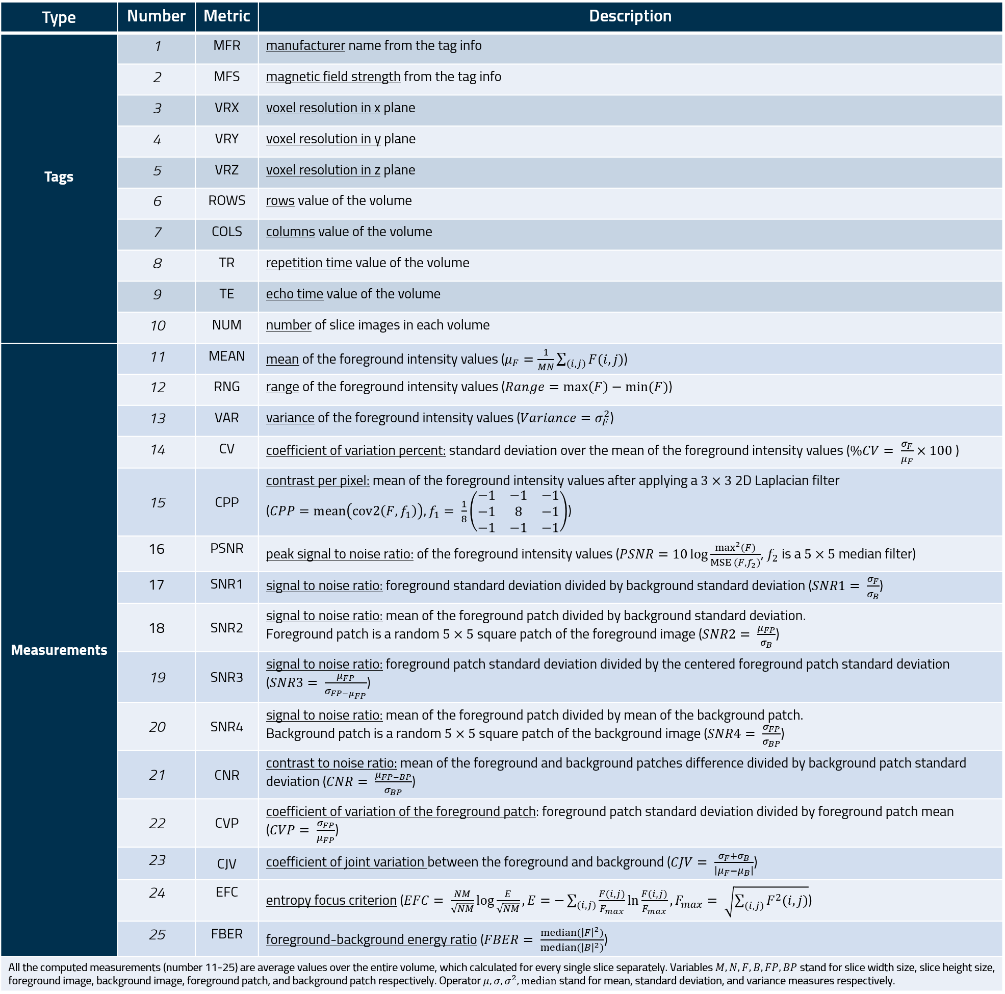
Table of metadata and measurements extracted.
The interactive user-interface of MRQy is built as a locally hosted HTML5/Javascript file (compatible with most popular web browsers such as Google Chrome, Firefox, and Chromium) that is specifically designed to enable real-time analytics, data filtering, and interactive visualization by the end-user. The goal is to allow end-users to easily investigate trends in site- or scanner-variations within an MRI cohort, as well as identify those scans that require additional processing due to the presence of artifacts. The MRQy interface splits into 3 major sections, all of which are inter-connected. Any individual section can also be disabled or re-enabled by the end-user to provide a fully customizable interface.
Extracted metadata and measures appear in separate tables within the interface. Each table has sortable columns to easily view outliers in numeric values. Any incomplete metadata values are displayed as "NA" (as well as being ignored in subsequent visualizations). Information can easily be copied out of the tables, which are also fully configurable including allowing for removal of specific subjects or specific columns.

Figure 2. Snapshot of both metadata and measures tables of the MRQy front-end. The highlighted row for patient ID TCGA-76-6663 is selected in both tables.
- Parallel Coordinate (PC): This is a multivariate visualization tool that has been shown to be effective for understanding trends within multi-variate datasets. For each MRI volume, a polyline is plotted (i.e. an unbroken line segment) which connects vertices of patient measurements on the parallel axes; i.e the vertex position on each axis corresponds to the value of the point for that specific metadata field or measure. The PC chart offers a visual approach to check variations in each measure as they related to the rest of the cohort as well as aid in the identification of outliers. If all the patients are consistent in all the measures, a series of straight lines would be plotted across all of the axes.

Figure 3. A snapshot of the PC chart. The yellow highlighted line corresponds to the selected row in Figure 2.
- Bar: A single bar is plotted per MRI volume for a selected variable (either metadata or measures). This provides an alternative approach to evaluating individual variables, where outliers would be markedly taller or shorter than the remainder of the cohort.

Figure 4. A snapshot of the bar chart. By clicking on the bar chart button in Figure 3 this plot will be shown. The yellow highlighted bar corresponds to the selected subject in Figures 2 and 3.
- Images: All the slices for a given patient volume are shown. Any outlier datasets can be quickly visually evaluated for obvious artifacts or issues.

Figure 5. A snapshot of the image section front-end.
To examine how the MRI volumes in a cohort relate to one another as well as to examine site- or scanner-specific trends, 2 different "embeddings" were computed based on the t-SNE and UMAP algorithms within the Python backend. Both these algorithms take as input all 23 measures for each patient and output a 2-dimensional embedding space (visualized as a scatter plot) where similarities between patients are preserved. While t-SNE yields a relatively robust representation of overall cohort structure, UMAP additionally provides a topological data structure for the cohort. t-SNE was implemented using the sklearn.manifold Python package with default parameters (e.g. n_components = 2, perplexity = 30, random_state = 0), while UMAP utilized the umap-learn Python package in the backend with default parameters (n_components = 1, n_neighbors= 15, min_dist= 0.1, metric = "euclidean"). These scatter plots are visualized based on the Plotly popular framework. Each panel has basic plot control functions.

Figure 6. Scatter plots and control tools. Highlighted nodes correspond to the selected patient from the Figures above.
By default, MRQy extracts a series of metadata information as well as image quality measures, as described above. Additional tag fields or private metadata can also be pulled from each scan based on specifying them via a .txt file input as follows:
python QC.py output_folder_name "input directory" -t "tags .txt address"
In addition, the user can supply a configuration for the foreground detection algorithm - either to detect objects separately or as a single object. By using the following command, the tool computes the foreground region for each image object separately:
python QC.py output_folder_name "input directory" -c "True"
The default value for the -c flag is False in which the whole body part is considered as the foreground mask.
Moreover, the user can specify if the foreground masks are needed to be saved or not by:
python QC.py output_folder_name "input directory" -s "True"
The default value for the -s flag is False in which the foreground mask won't save in the output directory.
The user can also work with the input folder names as the subject's ID. This functionality may be useful for the same subjects with different series of scans (e.g. in DICOM files). The syntax for this option is as follows:
python QC.py output_folder_name "input directory" -f "True"
The default value for the -f flag is False.
In some experiments applying a QC action over a fraction of the whole volume is needed. By the following command, one can force MRQy to analyze desired_value percent of the middle of the volume scans.
python QC.py output_folder_name "input directory" -u desired_value_percent
The default value for the -n flag is 100% in which the whole volume is considered as the input.
In order to have quick QC results, the user can run MRQy over some samples of the scans instead of all scans through the bellow command:
python QC.py output_folder_name "input directory" -b sample_size
The default value for the -b flag is sample_size = 1 in which all the scans are considered as the input samples.