Home

Processing in Detail (Diamond / CCP4 - 2023)

Introduction

DIALS processing may be performed in three possible ways:

• Running the individual tools on your terminal (spot finding, indexing, refinement, integration, symmetry, scaling, exporting to MTZ)
• Running the same tool from a graphical user interface (Dui2, this tutorial)
• Running xia2, which makes informed choices for you at each stage.

In this tutorial we will run through each of the steps with Dui2, taking a look at the outputs as we go. We will also look at enforcing the correct lattice symmetry. If you feel comfortable typing commands you may follow this command line tutorial instead, which processes in a very similar way from command line.

The aim of this tutorial is to introduce you to Dials and Dui2, not to teach about data processing. It is assumed that you have some idea of the overall process from e.g. associated lectures. We are not making so much of an effort to each command as simply "playing" with Dui2. This will give you a chance to learn your way around.

DIALS and Dui2 version

This tutorial assumes you are using and have set up DIALS version 3.17 and Dui2 version 2023.11.13 (i.e. you've run module load dui2).

If you are running this at home with a different version of DIALS or Dui2, details may change but the general flow should be the same.

Tutorial data

The data for this tutorial were collected with a deliberately wide-ish rotation angle (i.e. going against the advice in the lectures) to allow for quick processing. They are in

    /dls/i03/data/2023/mx37045-1/TestInsulin/ins_1/

Files

DIALS creates two principal file types:

• experiment files called something.expt
• reflection files called something.refl

"Experiment" in DIALS has a very specific meaning: the capturing of data from one set of the detector, beam, goniometer and crystal; if you have two scans from one crystal, this is two experiments; if you have two lattices on one data set, this is two experiments. In most cases you can ignore this distinction, though.

Working from inside a directory(folder)

When Dui2 runs, it needs to create some directories and files wherever it was called from, so it might be convenient for us to create a new directory ourselves and enter this new directory before launching Dui2. You can achieve this by typing:

    mkdir dui_work
    cd dui_work

Output

In the majority of cases, the DIALS programs will write their output to dials.program.log (e.g. dials.find_spots.log , etc.). Everything which is printed to the terminal is also saved in this file, so you can review the processing later. This is shown by Dui2 in the Log tab on the right half of the window. In the case where you are reporting an issue to the developers, including these log files in the error report (particularly for the step that failed) this log is very helpful.

From most stages, you can generate a more verbose report of the current state of processing with the dials.report command, which will generate a detailed report as an HTML file, this file is describing the current state of the processing. Dui2 will run dials.report automatically for you and show it in the Report tab right next to the Log tab on the right half of the window.

General workflow

The idea of Dui2 is to let you try to process data with DIALS in several ways and always let you go back to any previous point and retry. While you are running connected commands, there is a tree / flow graph that grows whenever a node is created. You can navigate to any node by clicking on it. Whenever you click on the button with an icon at the left hand side of the window, you create a new node that represents the new DIALS command ready to run. You can clone, run or stop any command with the three buttons that are at the bottom left of the window. While you are processing your data, Dui2 should look like this with a similar or bigger tree/flow

Now we are going to process an insulin data set without forking the tree / flow graph too much. If you are already in the directory created for processing with DIALS and your environment is already setup, you should just type:

    dui2

then the terminal will print some messages and eventually display a GUI that should look like this:

If after you type dui2 the terminal prints you a message like bash: dui2: command not found instead of showing a GUI, maybe it was not loaded during the execution of module load dui2. or something went wrong with either the installation of DIALS or Dui2

Import

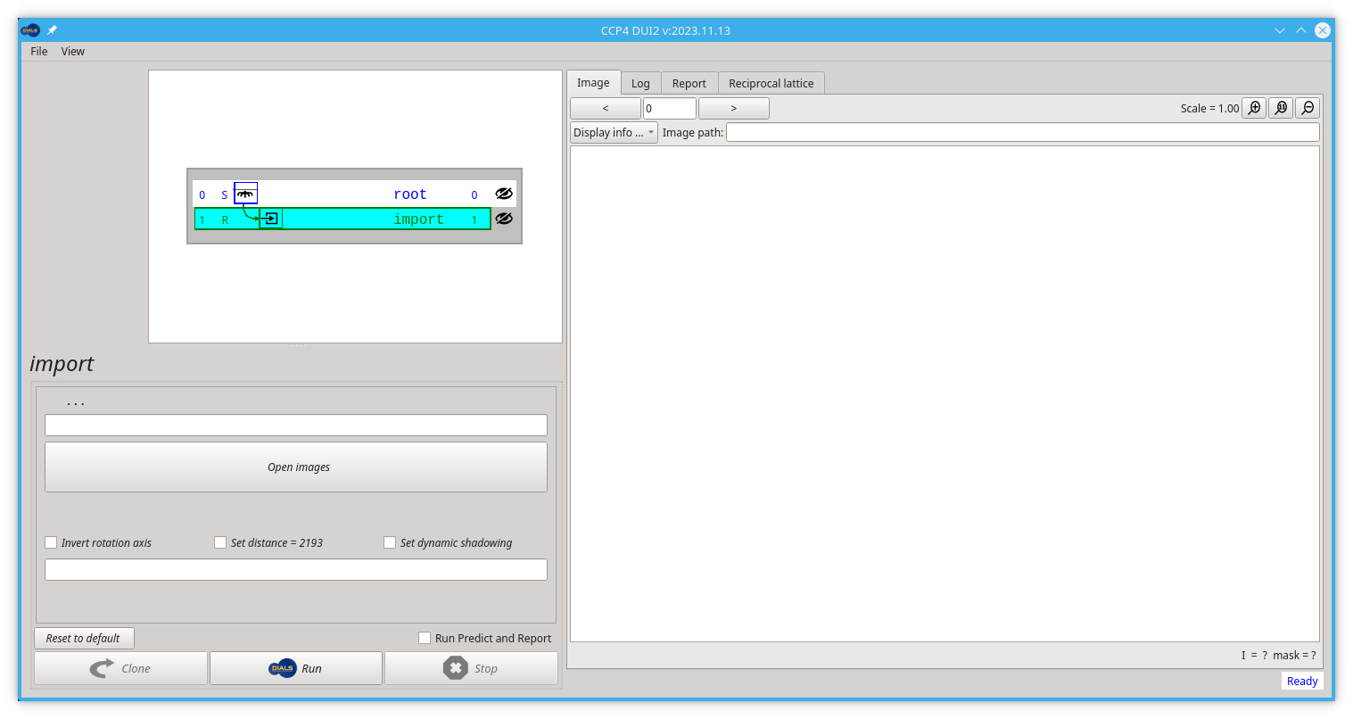
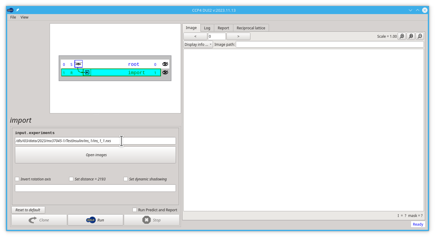
The starting point for any processing with DIALS is to import the data, here the metadata is read and a description of the data is to be processed and saved to a file named imported.expt. This is "human readable" in the sense that the file is in the JSON format (roughly readable text with brackets around to structure for computers). While you can edit this file if you know what you are doing, usually this is not necessary and Dui2 reads and interprets this file for you.

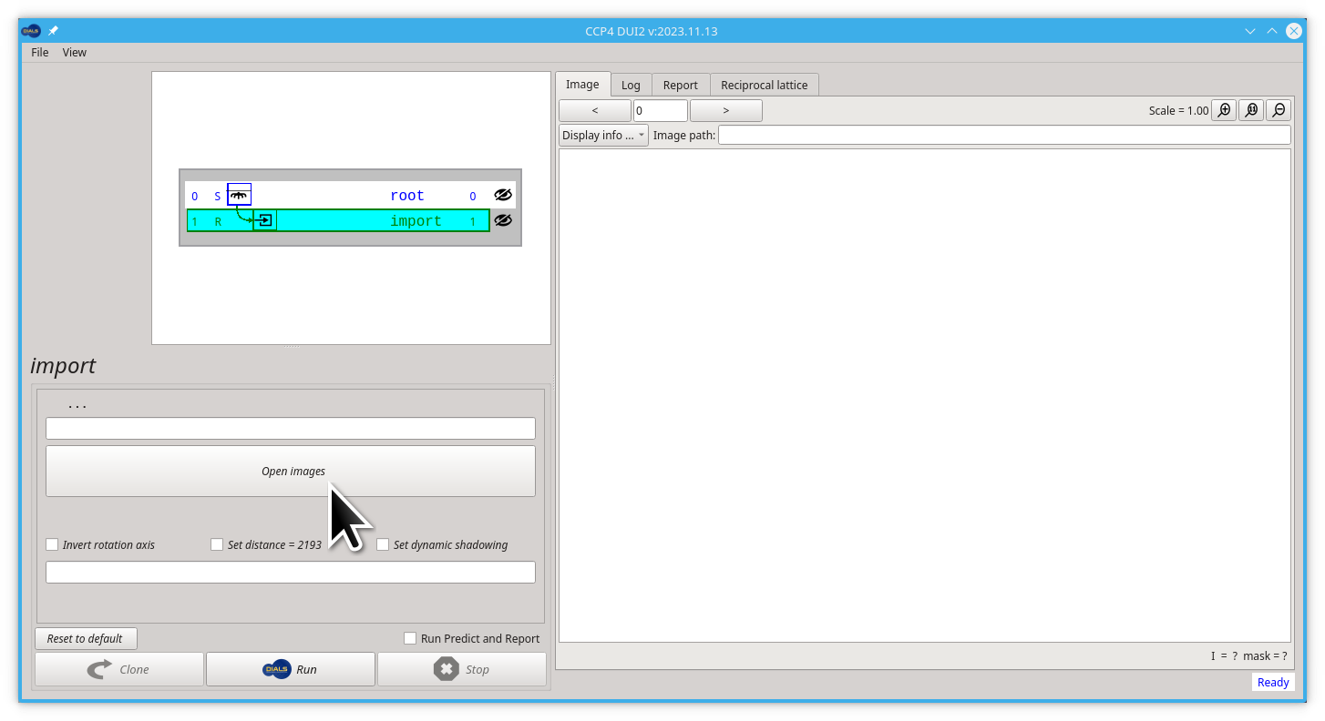
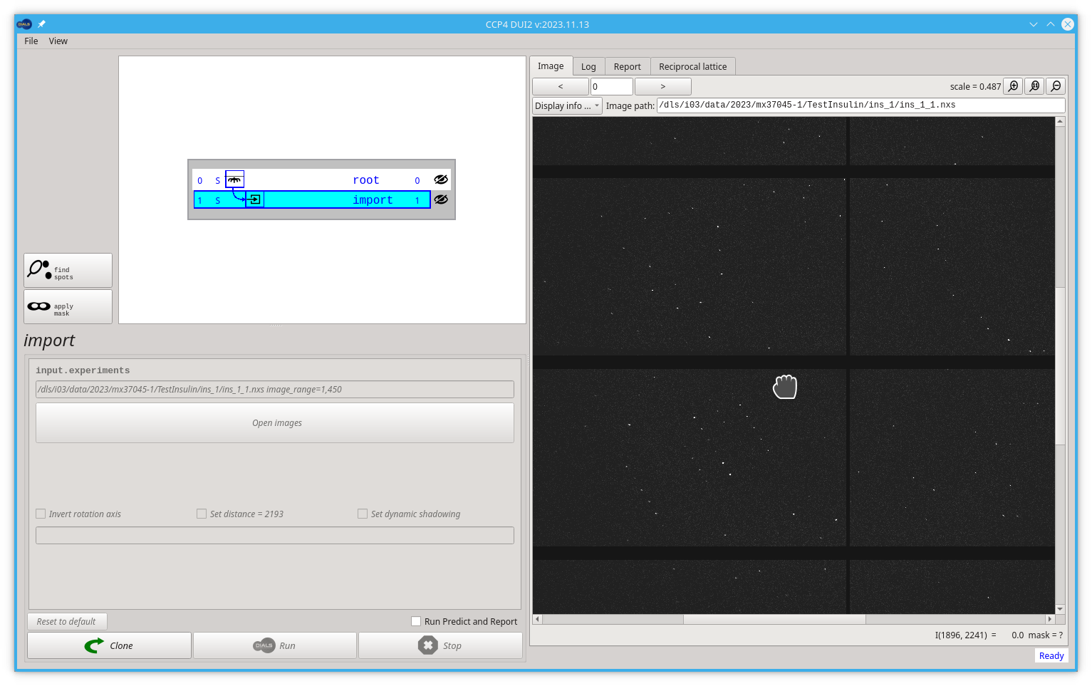
You should start by clicking the Open images button

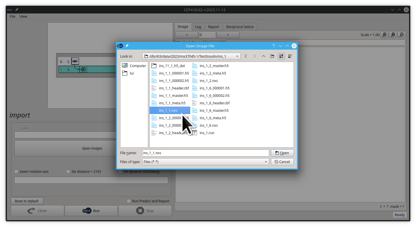
Then navigate to the path /dls/i03/data/2023/mx37045-1/TestInsulin/ins_1/ and select the file ins_1_1.nxs .

After selecting our .nxs file the Dui2 shoul look like this:

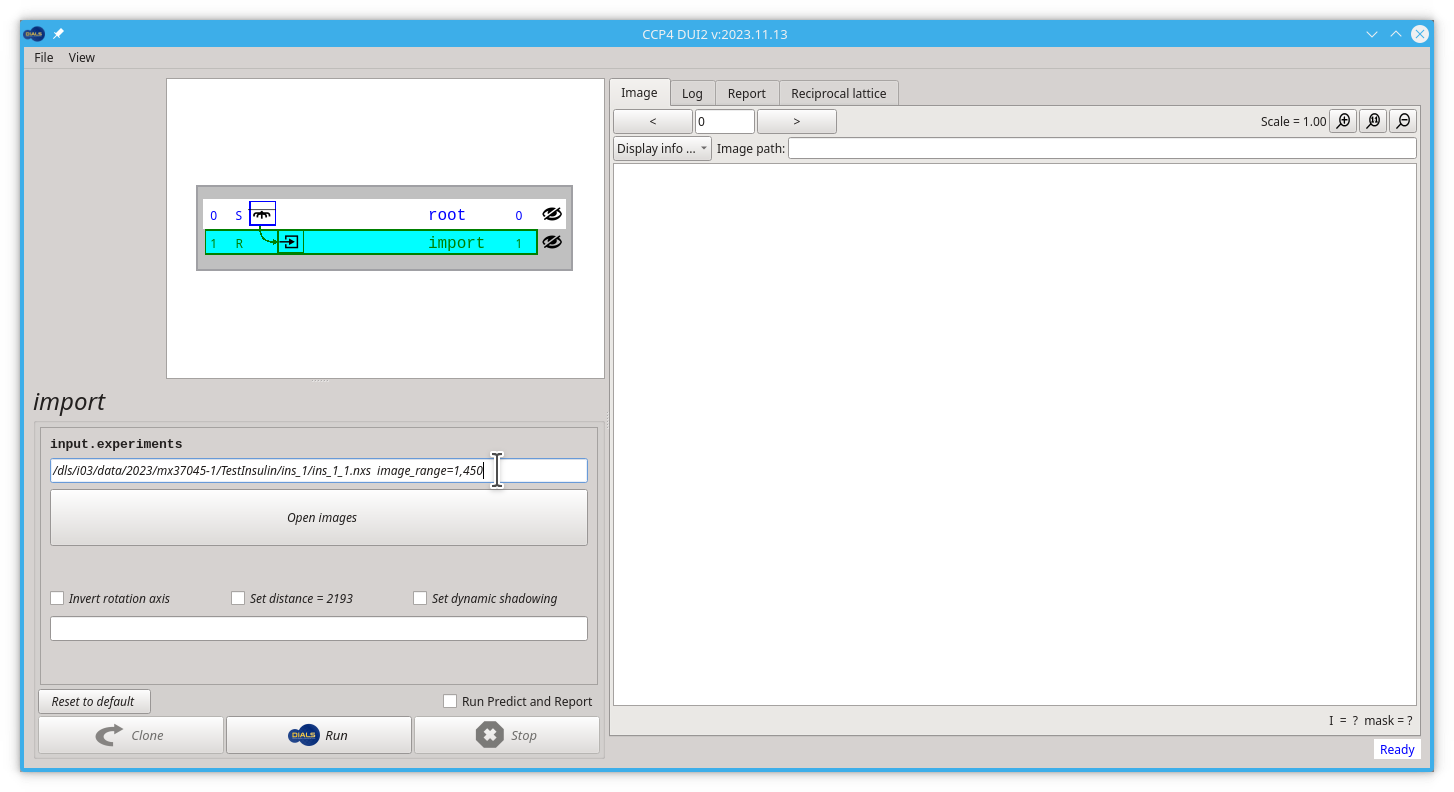
Now, before running the first DIALS command (dials.import) we are going to edit and tweak the way we import our data. For the purpose of speeding up the subsequent steps we are trimming our image range to only 450 images. This is rarely needed when we are processing with the intention of obtaining our structure in real life. For this particulas case, we are going to add the following parameter to the input text, you may copy/paste from this tutorial:

    image_range=1,450

remember to add an empty space between the file path and the new parameter, now Dui2 should look like this:

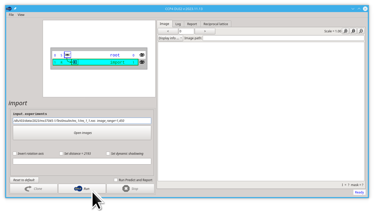
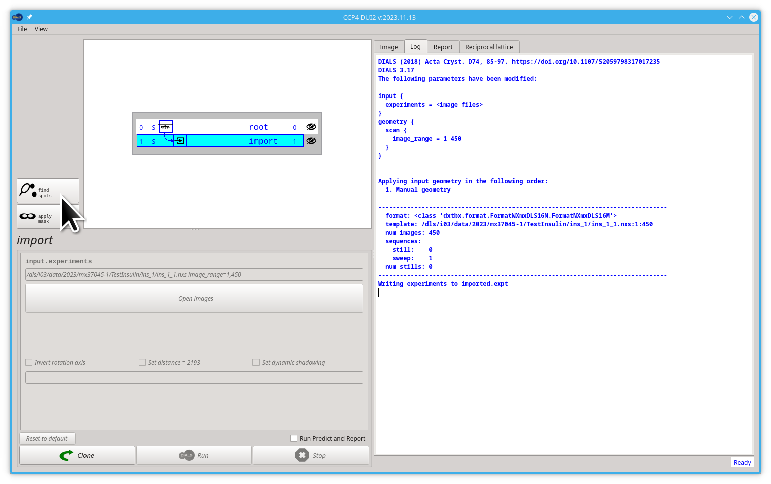
Now when you click the Run button, Dui2 will launch the dials.import command, which reads the metadata from this nexus file and writes imported.expt from this.

It is important to note that for well-behaved data (i.e. anything which is well-collected from a well-behaved sample) the steps to follow below will often be identical after importing.

Here is a short discussion on some more details on importing data.

After a successful import step, Dui2 should show the first image inside the Image tab. The Default minimum and maximum limits of the palette used to see the image will not be suitable for all possible images, so it is better to adjust the limits to our images. A good first approach would be to change the maximum limit from 50 to 20, as shown below.

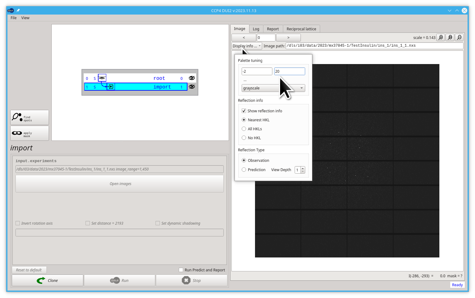
The image viewer inside Dui2 behaves very similar to "Google Maps" as you can drag the image (press, move, release) to move it, and you can zoom in and out by scrolling (mouse wheel or two fingers move on a touch-pad). You can play with the position and scale of your images. Try to see some diffraction spots like in the following image.

The Log tab on the right side of the window shows in real time the output of the DIALS commands. It shows valuable information about our sample and how the data processing goes. We will use this tab very frequently from now on. For example, after import it shows how we modified the parameter image_range to 1 450.

Find Spots

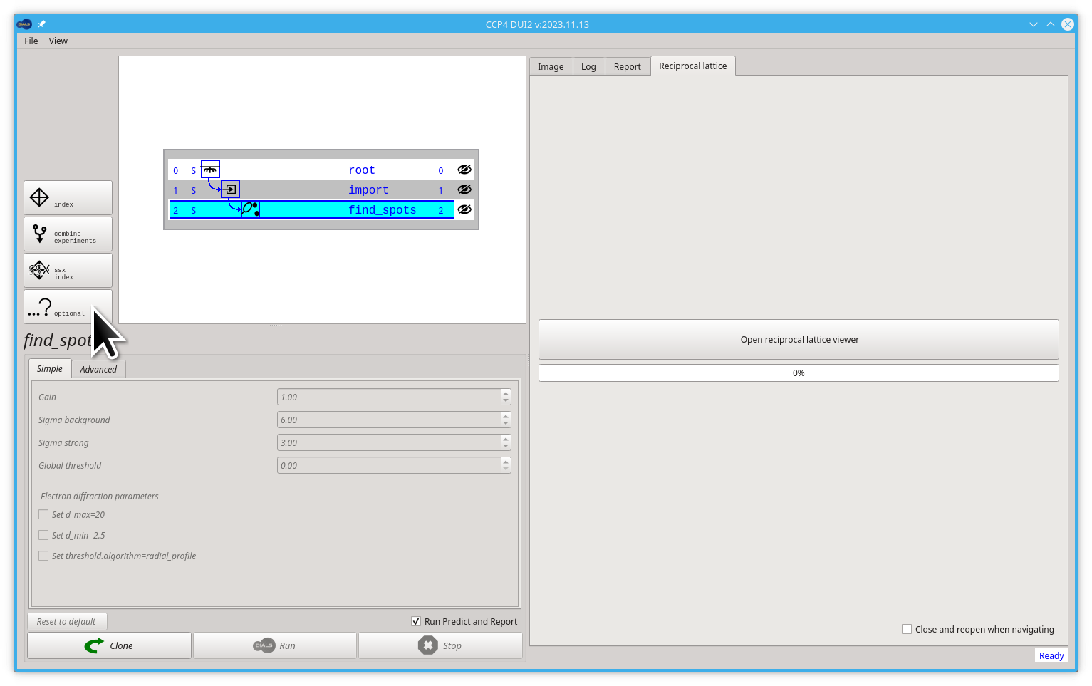
The next step will be spot finding, which is also the first "real" task in any processing using DIALS. Now you should click the find spots button.

Dui2 should create the new find_spots node.

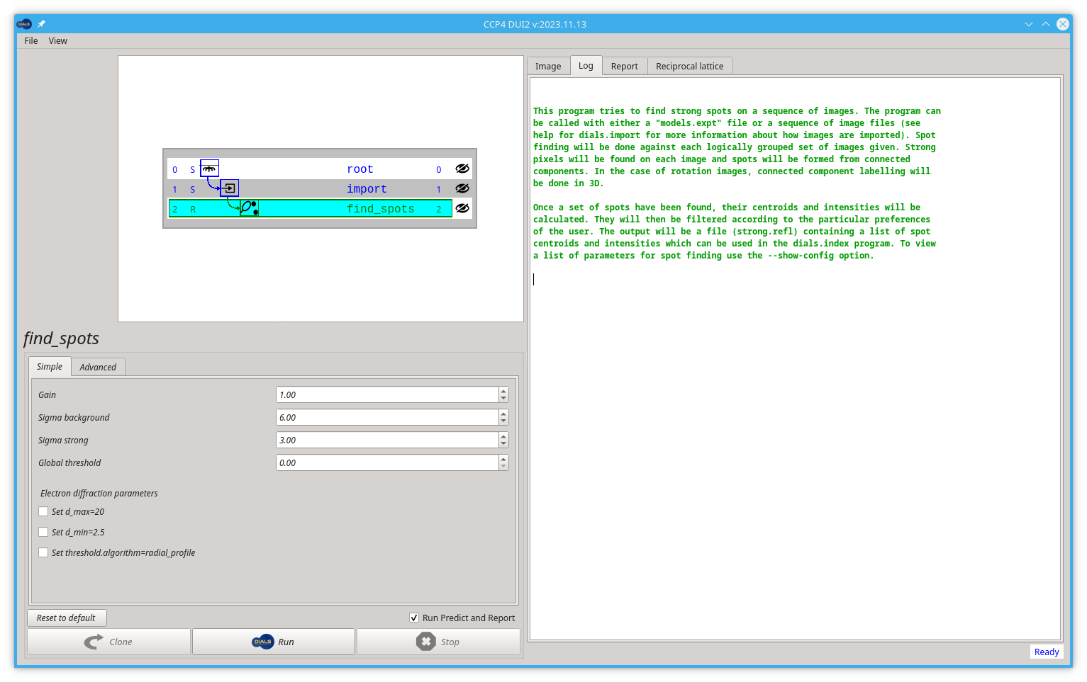
Since this task is looking for spots on every image in the dataset, this process can take some time so it will use all of the processors available on your machine by default. If you would like to control this, adjust with the parameter nproc=4 in the Advanced parameters tab. However, the default is usually sensible if you are not sharing the computer with many others.

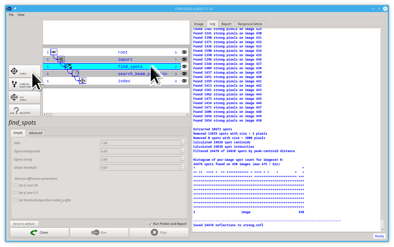
By clicking the Run button, you will ask Dui2 to launch the dials.find_spots command. After clicking, be patient, it will take a while.

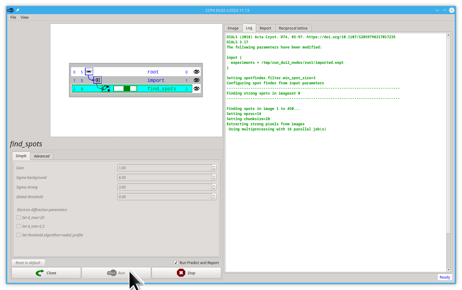
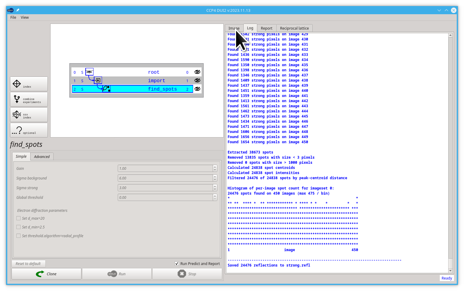
This is one of the two steps where every image in the data set is read and processed and hence can be moderately time-consuming. This contains a reflection file called strong.refl which contains both the positions of the strong spots and also "images" of the spot pixels which we will use later.

After it finishes with find spots, we should see the text-based histogram of spots found per image in the log tab and the fonts should change to blue.

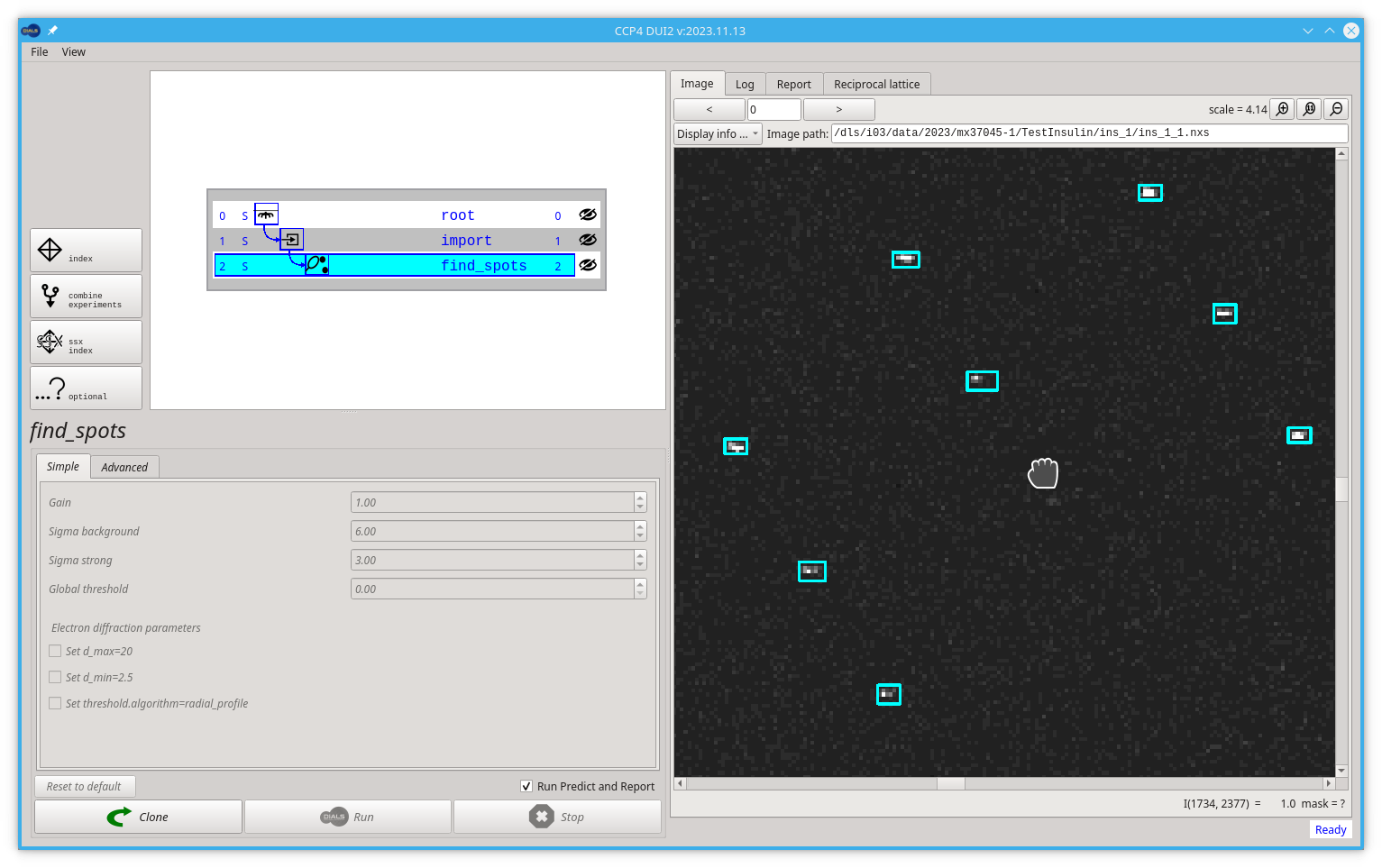
You can now click on the Image tab to see some result on the images.

In the image viewer, remember that you can drag to move the image and scroll to zoom. Try to find some rectangles around the spots, these are the bounding boxes of the reflections i.e. the outer extent of the connected regions of the signal pixels.

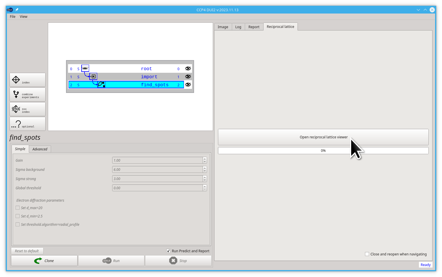
There is a command line tool in DIALS for visualisation of the found spots mapped to the reciprocal space.

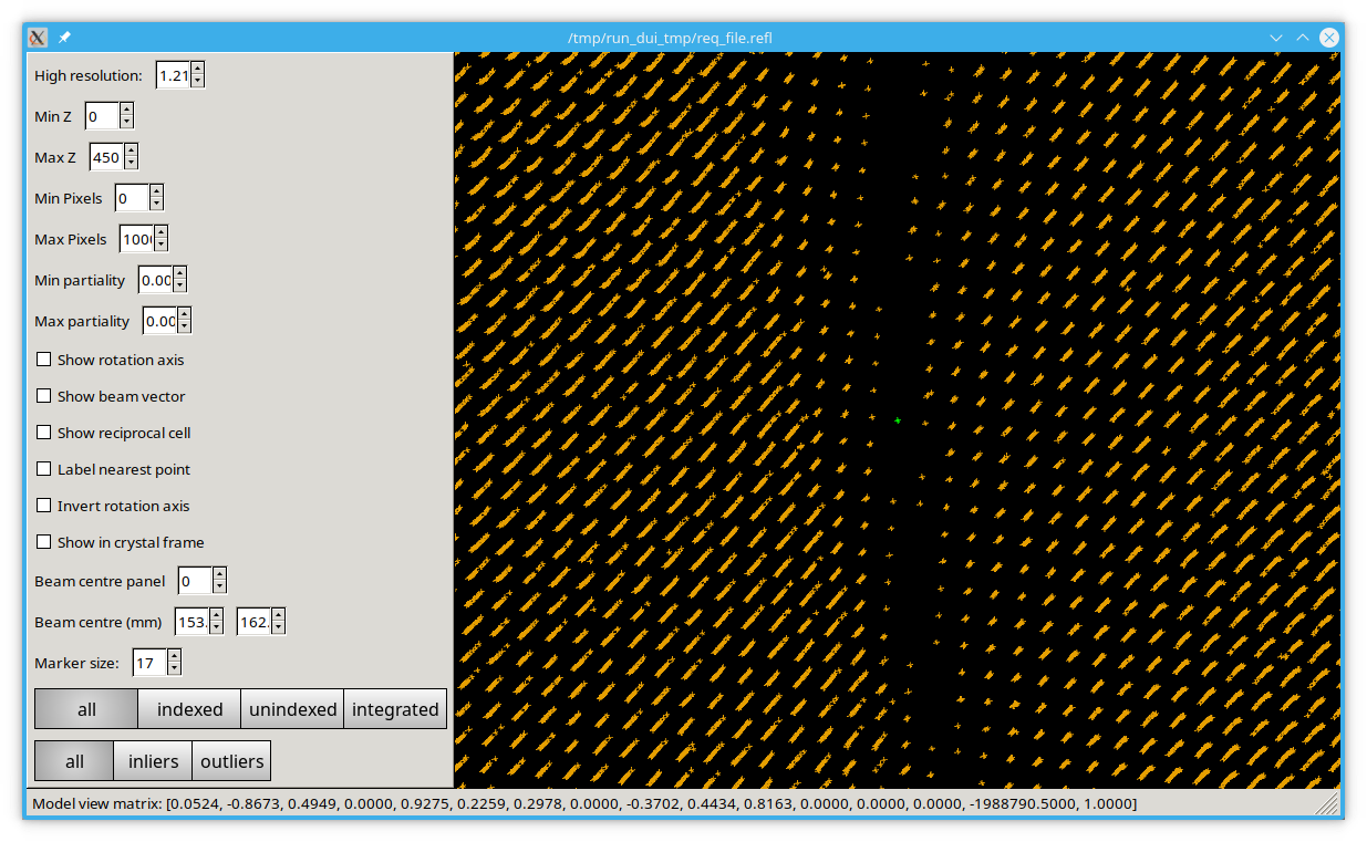
To open this viewer you should click on the Reciprocal Lattice tab then click the Open reciprocal lattice viewer button.

No matter the sample orientation, you should be able to rotate the space to "look down" the lines of reflections. If you cannot, or the lines are not straight, it is likely that there are some errors in the experiment parameters e.g. detector distance or beam centre. If these are not too large they will likely be corrected in the subsequent analysis.

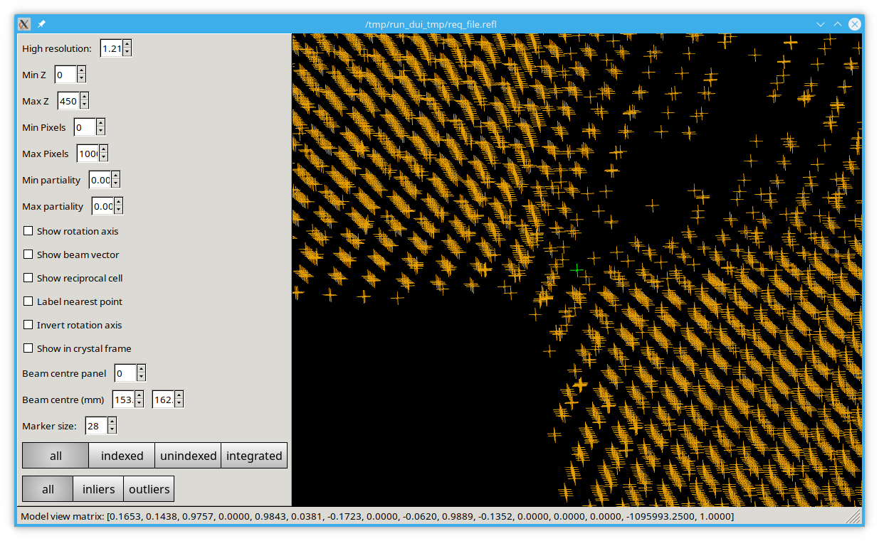
Have a play with the settings, you can change the beam centre in the viewer to see how nicely aligned spots move out of alignment. Some of the options will only work after you have indexed the data.

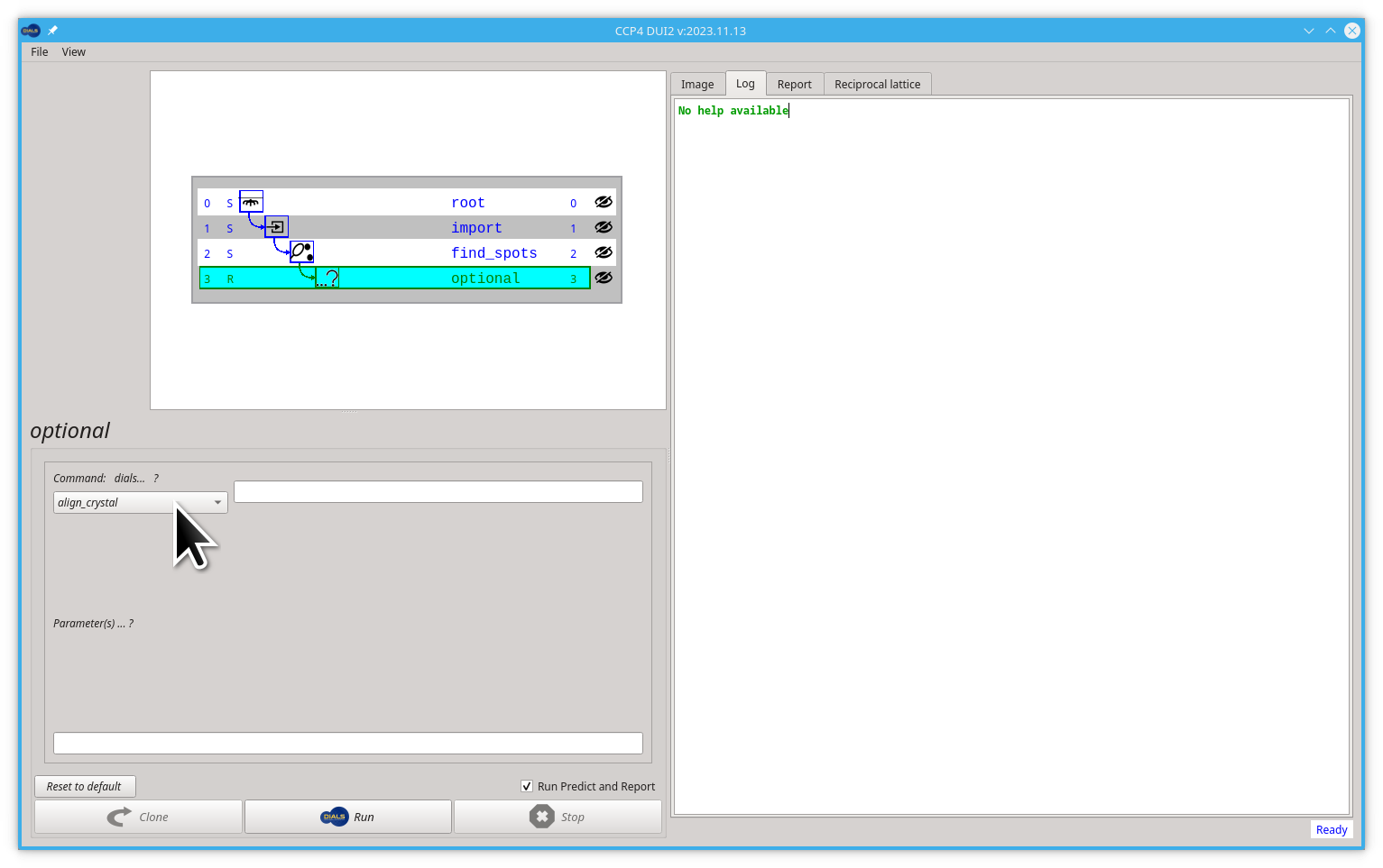
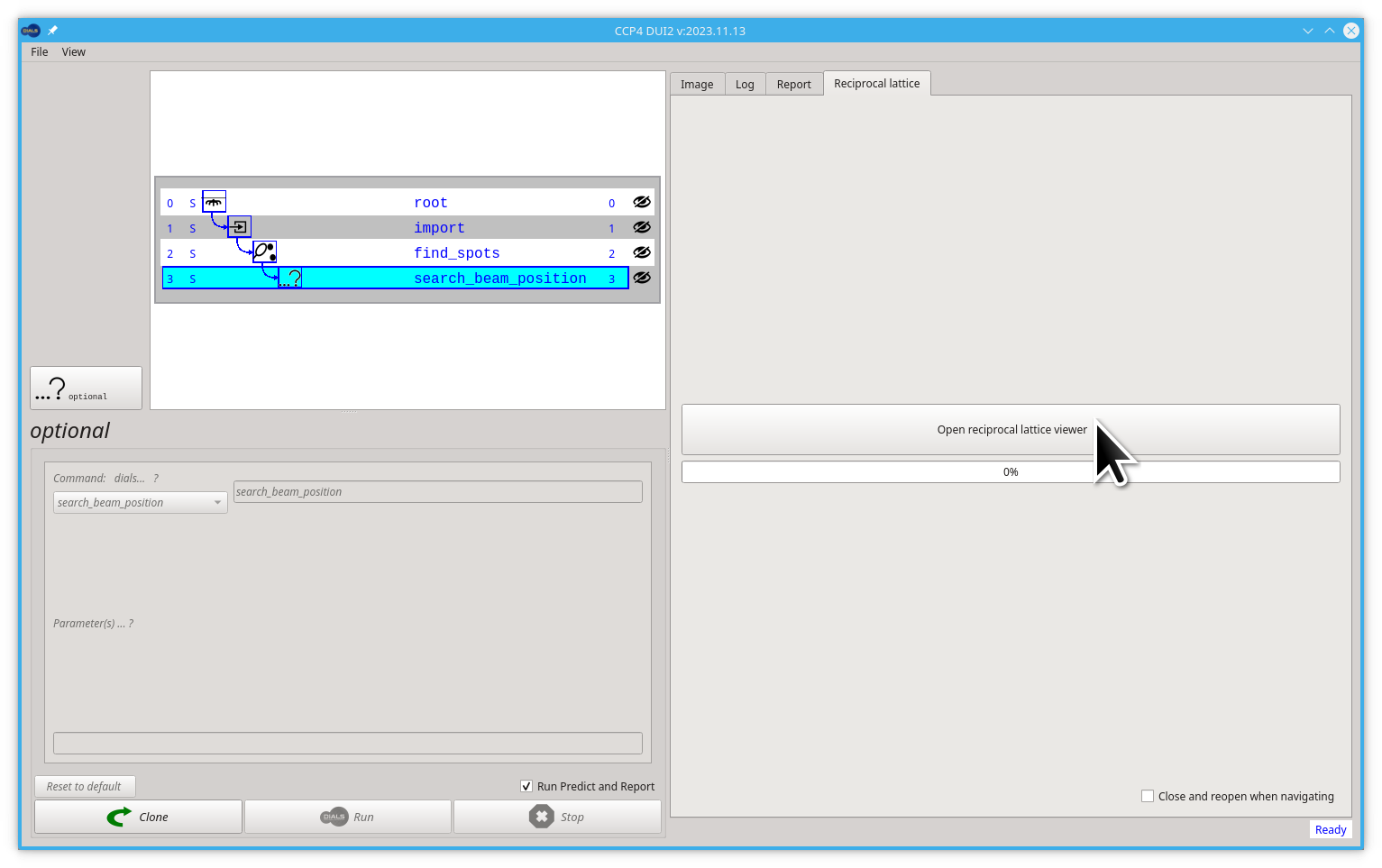
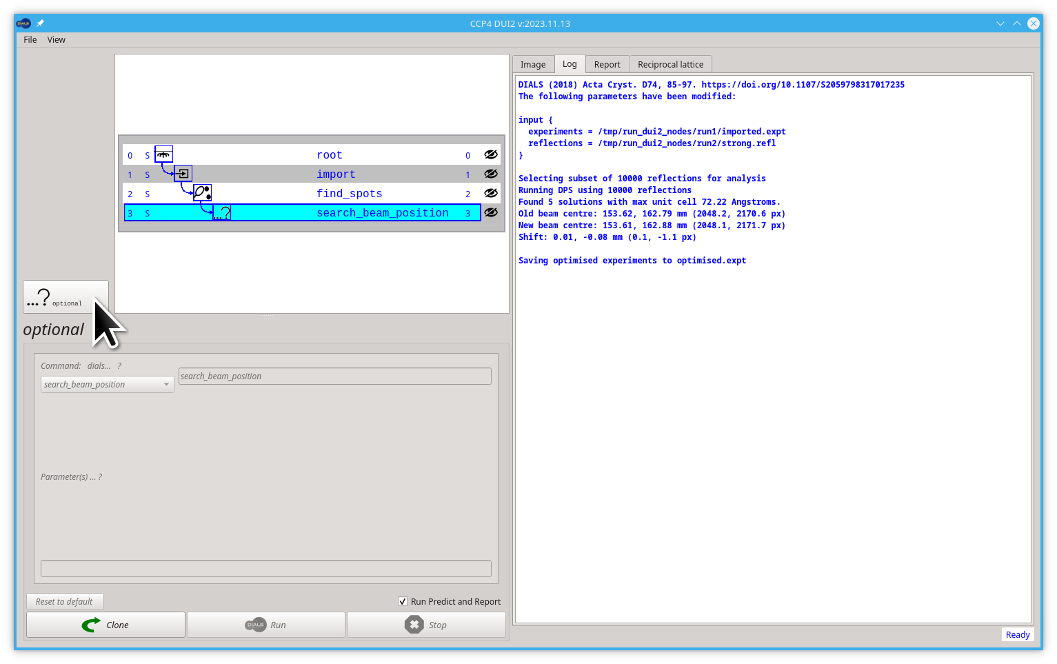
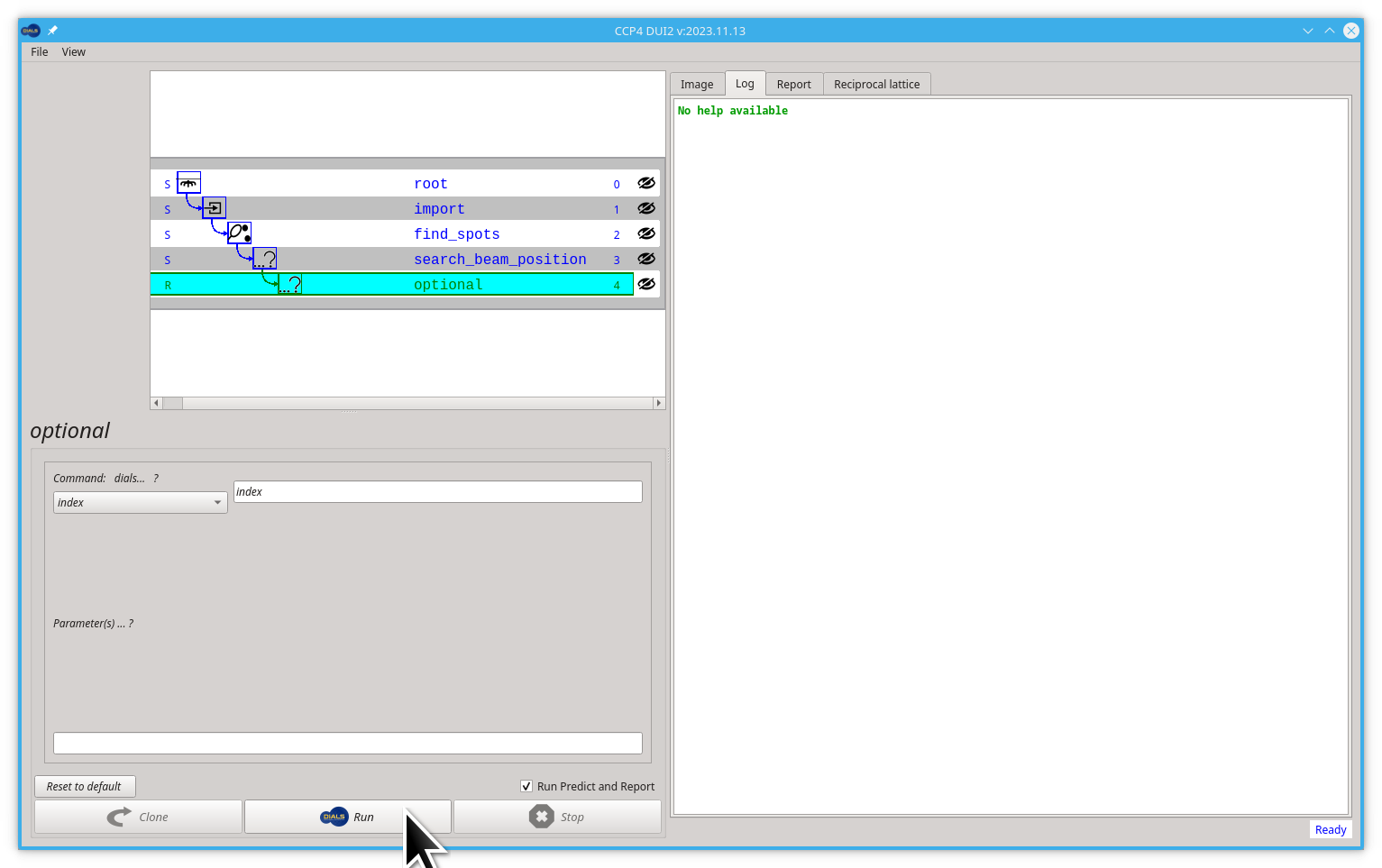
Sometimes we find that if the geometry in our experiment is not accurately recorded. In that case, you may find it useful to run dials.search_beam_position. This is not a very frequently used command, that's why it is in the "? optional" command list. Let's run this command now, start by clicking the optional button then change to the Log tab.

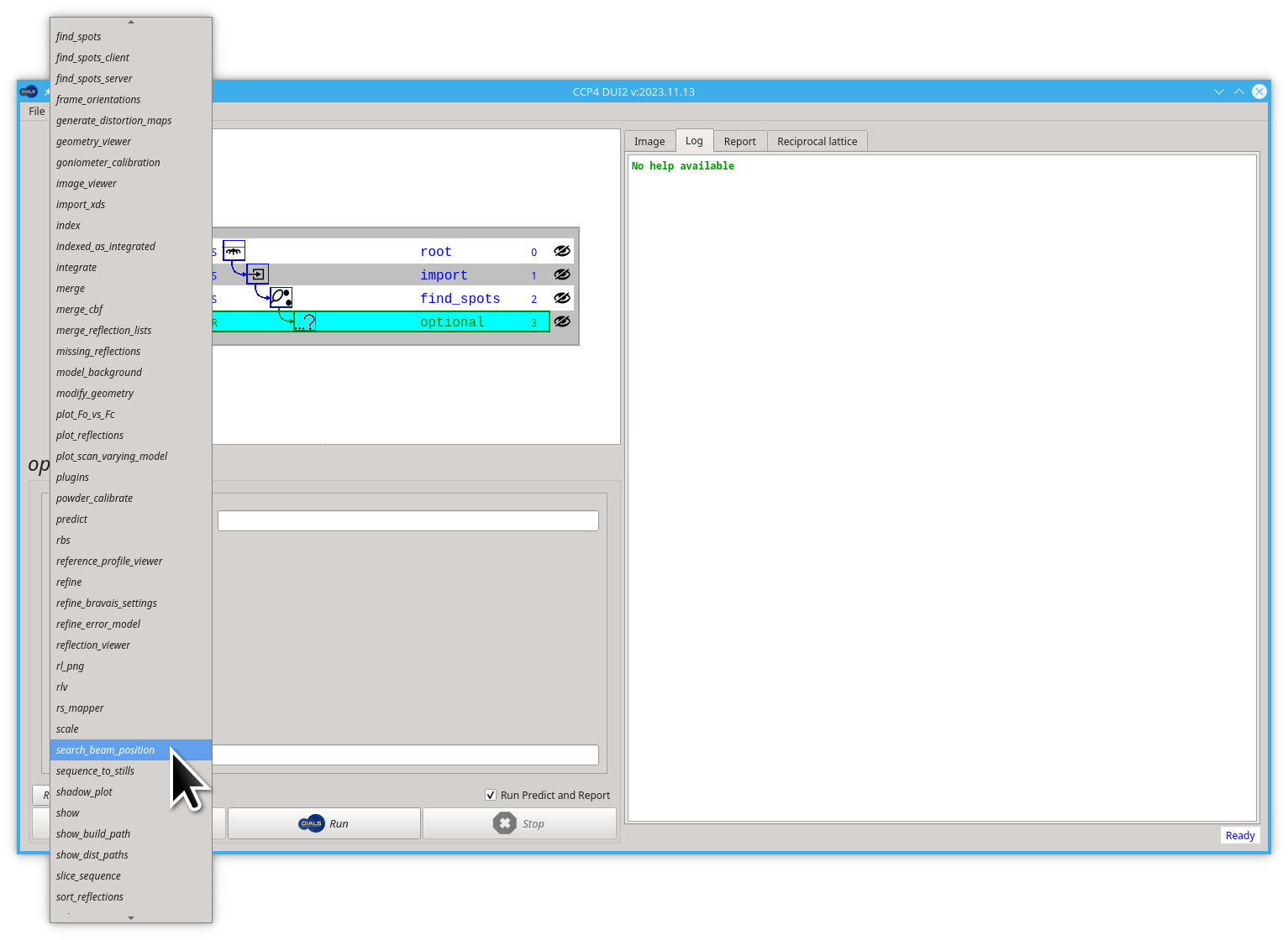
Now you should pick the option search_beam_position from the pull-down menu bellow the label Command: dials... ?

It worth noticing that the menu is bigger than the screen so you will need to scroll down to find the search_beam_position option

Now click on the Run button to launch the dials.search_beam_position command

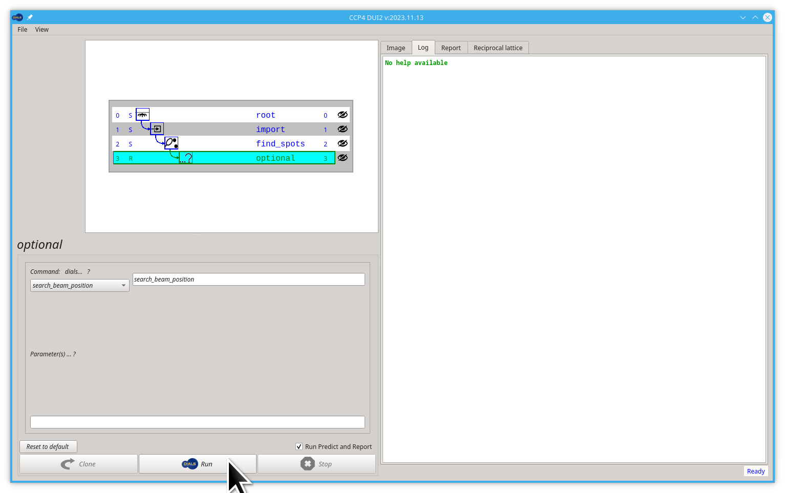
to determine an updated position for the beam centre. The shift that this calculates should be small if the beamline is well-calibrated and if it is bigger than a couple of mm or more it may be worth discussing this with the beamline staff! Again, click on the Reciprocal lattice tab then click on the Open reciprocal lattice viewer button

Running the reciprocal lattice viewer with the optimised experiment output should show straight lines, provided everything has worked correctly.

Indexing

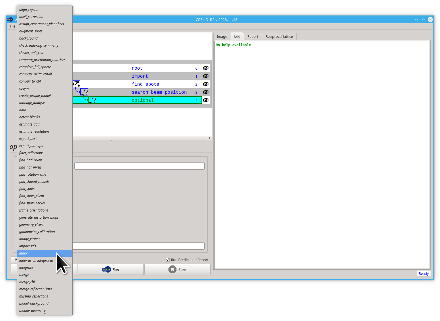
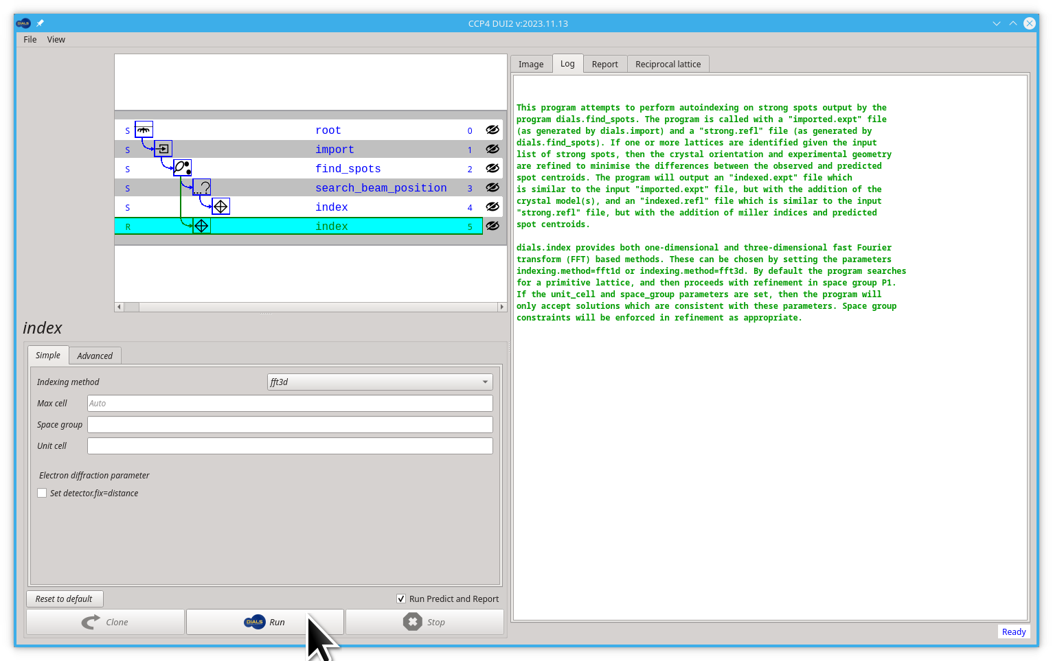
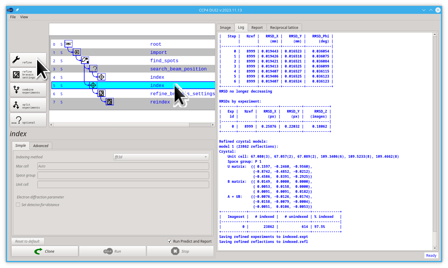
The next step will be indexing of the found spots with dials.index. By default this uses a 3D FFT algorithm to identify periodicity in the reciprocal space mapped spot positions, though there are other algorithms available which may be better suited to specific circumstances. For example, for narrow data sets, the 1D FFT algorithm may be better. To run dials.index.

to run any DIALS command after an optional node you should click again the same optional button and then select in the menu as before.

Next we are going to select the index option.

As any other command used for processing data we should click on the Run button.

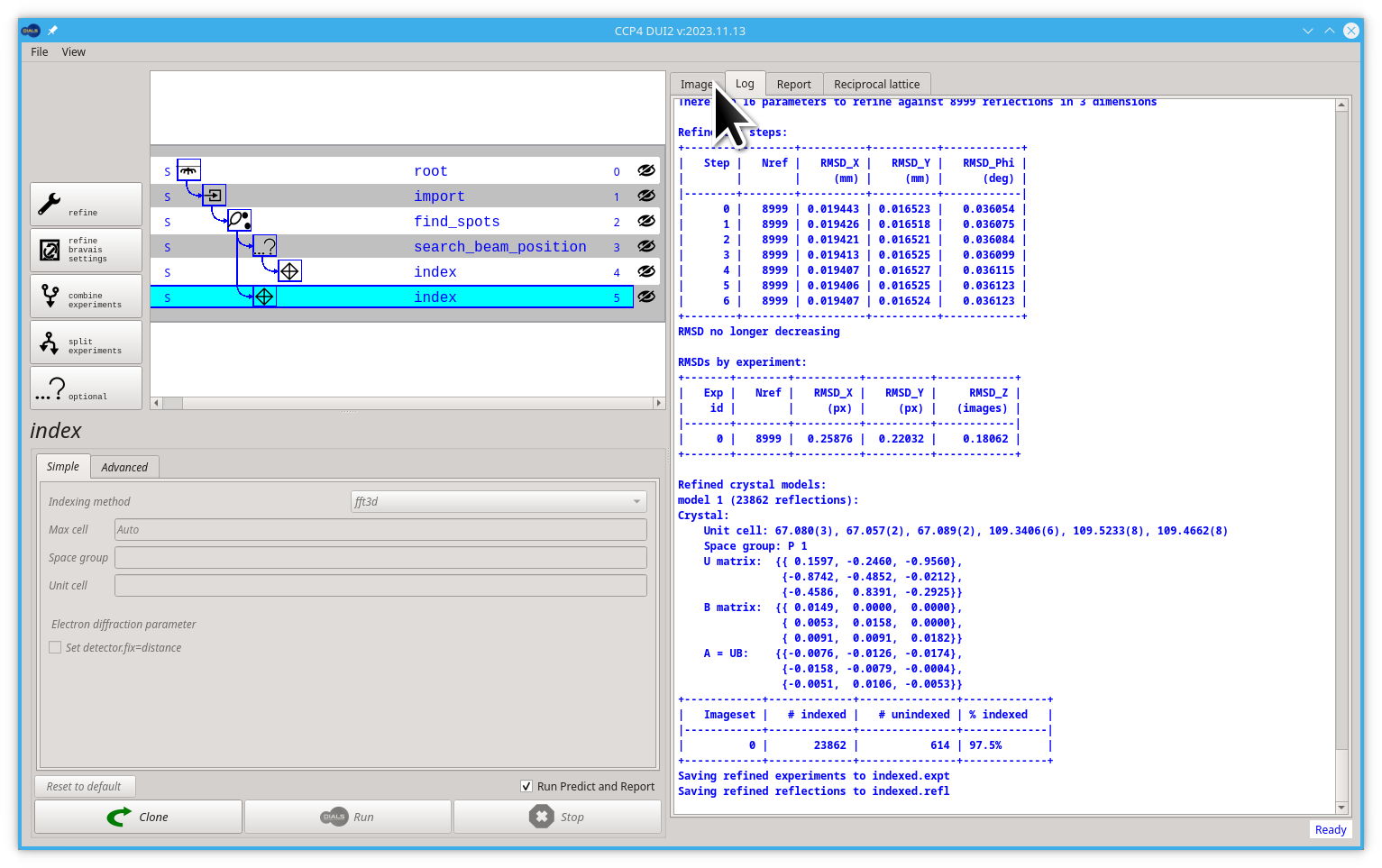
The most common parameters to set are the space_group and unit_cell if these are known in advance. While this does index the data, it will also perform some refinement with a static crystal model and indicate in the output that the fraction of reflections which have been indexed (ideally this should be close to 100%):

Luckily in this example we are close enough to 100, if not we should consider treating the data as a multicrystal dataset. That would be a different tutorial.

The process that the indexing performs is quite complex -

• make a guess at the maximum unit cell from the pairwise separation of spots in reciprocal space
• transform spot positions to reciprocal space using the best available current model of the experimental geometry
• perform a Fourier transform of these positions or other algorithm to identify the basis vectors of these positions e.g. the spacing between one position and the next
• determine a set of these basis vectors which best describes the reciprocal space positions
• transform this set of three basis vectors into a unit cell description, which is then manipulated according to some standard rules to give the best triclinic unit cell to describe the reflections - if a unit cell and space group have been provided these will be enforced at this stage
• assign indices to the reflections by "dividing through" the reciprocal space position by the unit cell parallelopiped (this is strictly the actual indexing step)
• take the indexed reflections and refine the unit cell parameters and model of the experimental geometry by comparing where the reflections should be and where they are found
• save the indexed reflections and experiment models to the output files

The indexing process takes place over a number of cycles, where low resolution reflections are initially indexed and refined before including more reflections at high resolution - this improves the overall success of the procedure by allowing some refinement as a part of the process.

During this process an effort is made to eliminate "outlier" reflections - these are reflections which do not strictly belong to the crystal lattice but are accidentally close to a reciprocal space position and hence can be indexed. Most often this is an issue with small satellite lattices or ice / powder on the sample. Usually this should not be a cause for concern.

Forking the tree/graph

Let's suppose we don't like the way our processing is going, this when we can fork our path, remember that you can always go back to any node in the tree/graph. Let's suppose we want to run dials.index without running dials.search_beam_position. Start by clicking on the find_spots node, then click the index button again.

We have already forked our path. Now you may click the Run button.

After some processing, Dui2 should look like the following image. Let's have a look at the images and see some results of our processing in this node. Click on the Image tab

The image viewer should behave just like before, you can still "drag" and "scroll" if you want to move or zoom your image, but now, after indexing, Dui2 should show you the Miller indexes of the reflection closest to the mouse pointer. You can ask it to show you all the Miller indexes for every reflection. Click on the Display info pull-down menu, then select All HKL option.

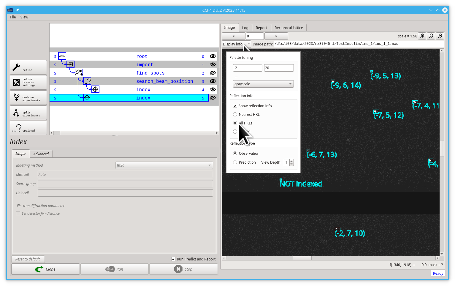
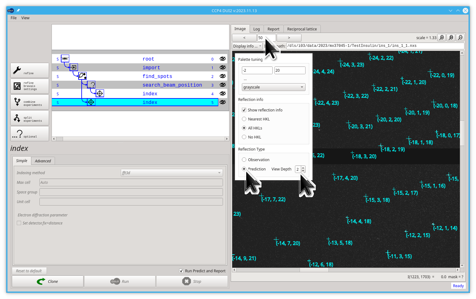
There is a dials.predict command that, from the current model, calculates the position of every reflection corresponding to a desired step in our processing path. Dui2 runs this command automatically after every step. You can see the predicted reflections by selecting the Prediction option in the pull-down menu. You should keep in mind that for every reflection, the prediction is in a unique place in a single frame, so to find some similitude between your experimental image and the predictions, you should play with the image number and the depth of our representation.

Try jumping to image 50 (press Enter) and increasing the View Depth to 2

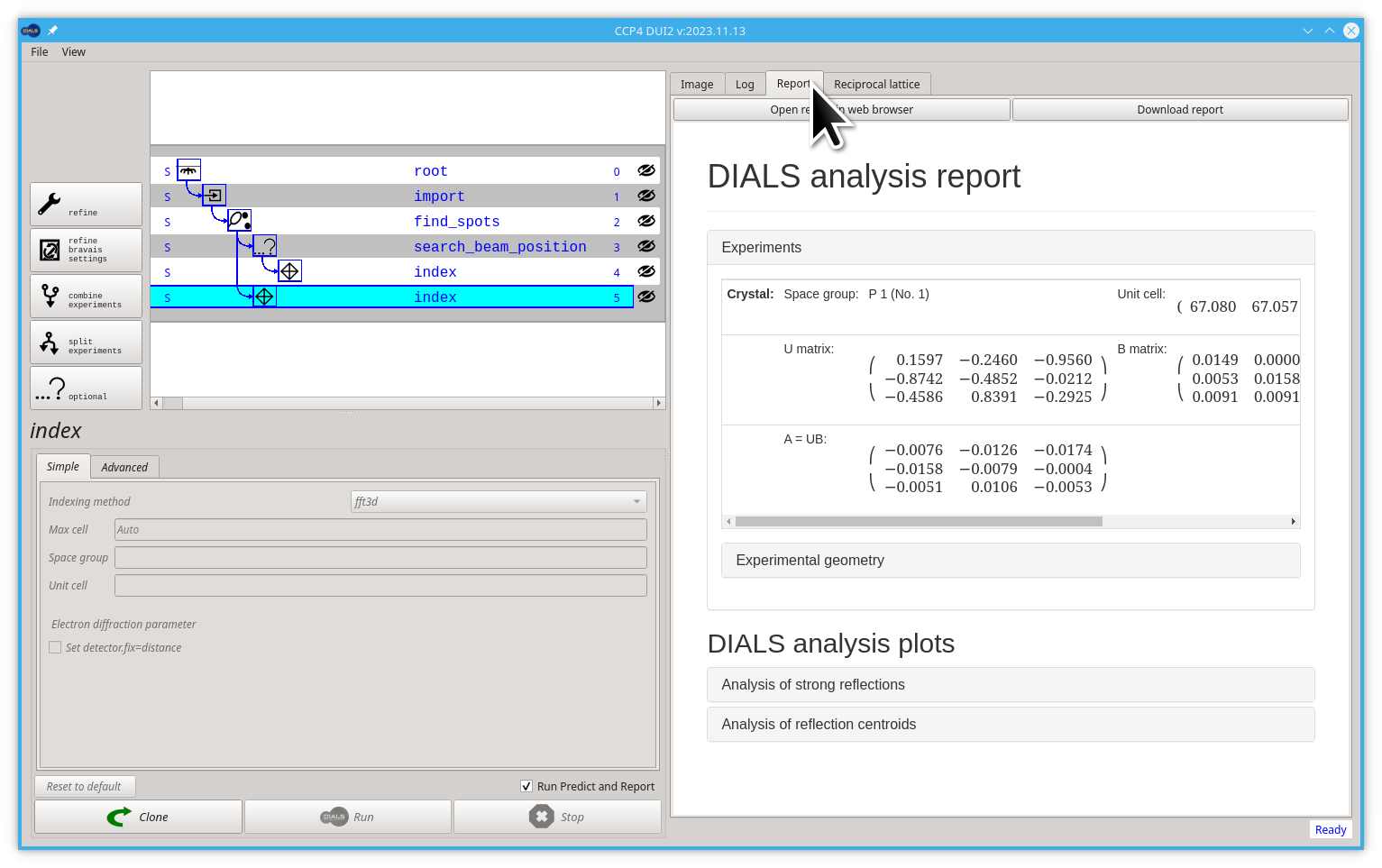
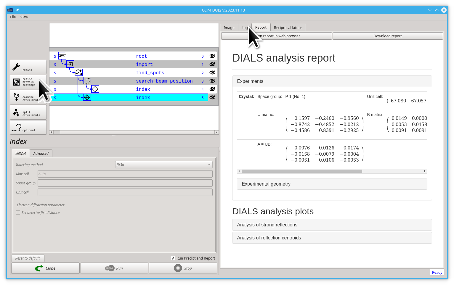
We can also have a look at the HTML report generated by dials.report if we click on the Report tab. There is a lot of information on this report, feel free to look around but explaining all the context of this report is enough for another tutorial.

Bravais Lattice Determination (optional!)

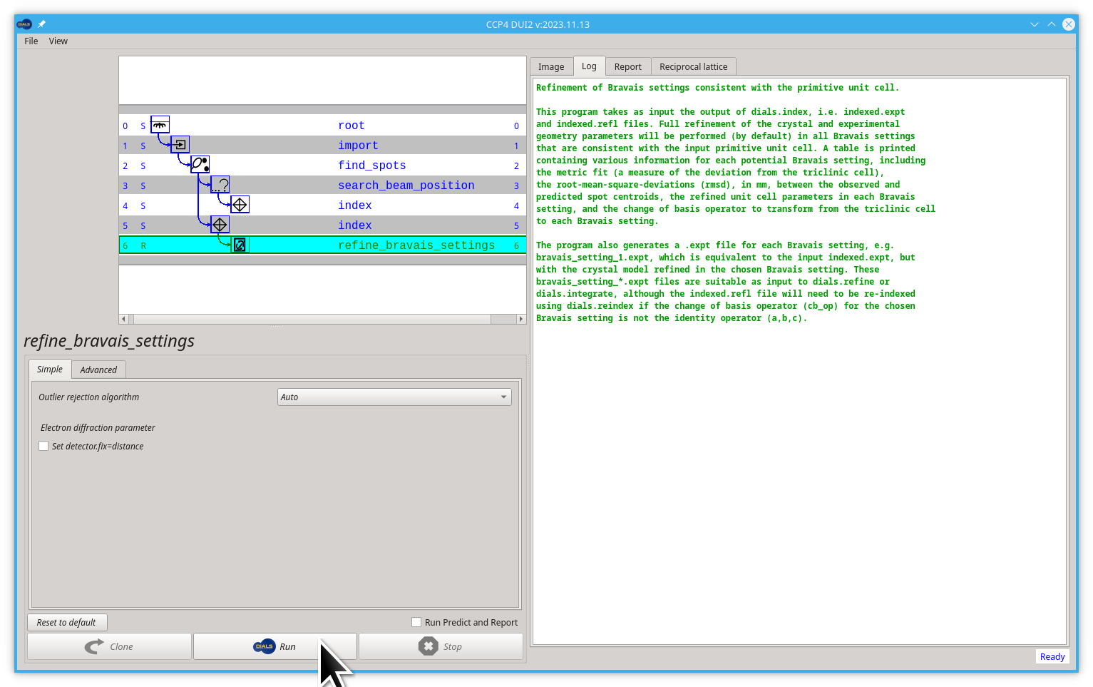
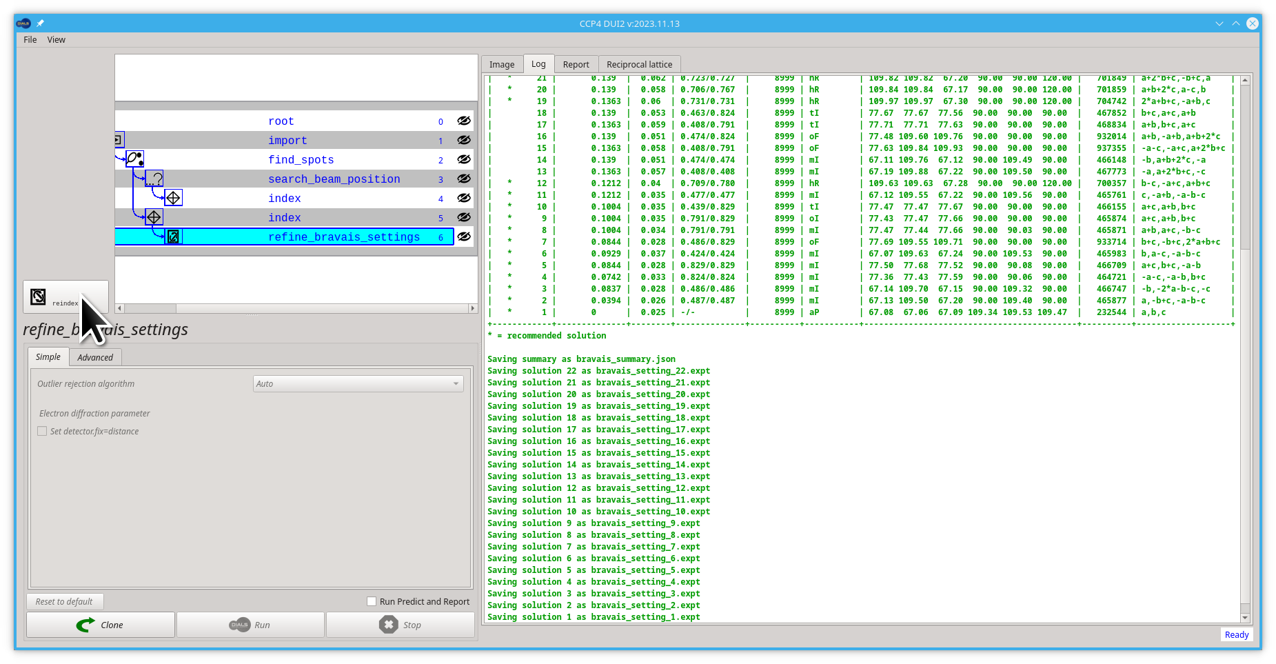
Once you have indexed the data, you may attempt to infer the correct Bravais lattice and assign this to constrain the unit cell in subsequent processing but this is optional. If, for example, the unit cell from indexing has all three angles close to 90° and two unit cell lengths with very similar values, you could guess that the unit cell is tetragonal. In dials.refine_bravais_settings we take away the guesswork by transforming the unit cell to all possible Bravais lattices which approximately match the triclinic unit cell, and then performing some refinement (if the lattice constraints are correct, then imposing them should have hardly any impact on the deviations between the positions of the observed and calculated reflection known as the R.M.S. deviations). If a lattice constraint is incorrect, it will manifest as a significant increase in deviation. However, care must be taken as it can be the case that the true symmetry is lower than the shape of the unit cell would indicate.

In the general case, there is little harm in skipping this step. However, for information purposes only, if you want to try it, follow the next steps:

• Go back to Log tab and click on the refine bravais settings button

• Click the Run button

you will see a table of possible unit cell / Bravais lattice / R.M.S. deviations printed in the output. In the case of this tutorial's data, they will all match, as the true symmetry is tetragonal.

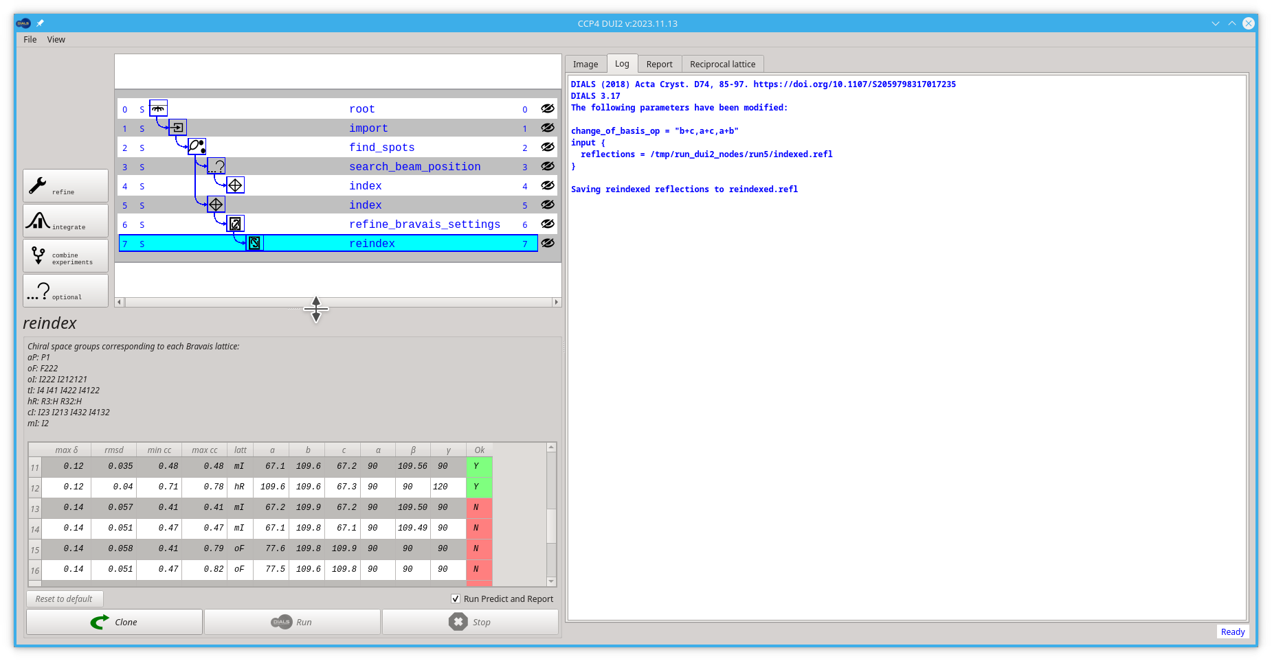
If you wish to use one of the output experiments from this process (e.g. bravais_setting_22), you will need to:

• Click the Reindex button

• Scroll down or "enlarge" the table viewing area

• Double click the lowest option on the table, or click on the lower option and then click the Run button

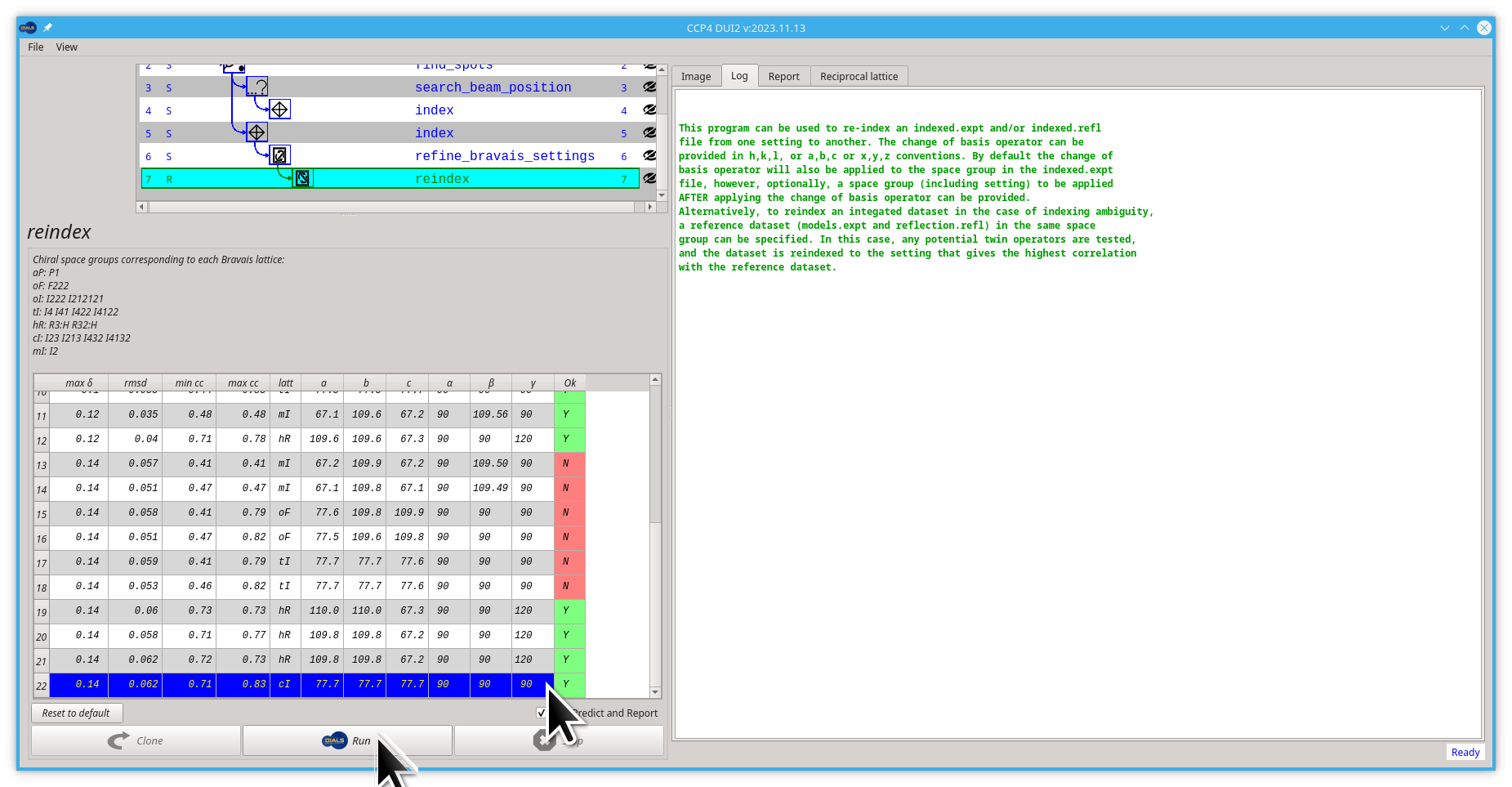
• Pull back the viewing area to a smaller size so you can see the new reindex node in the tree/graph

The reader is reminded here that in most cases it is absolutely fine to proceed at this stage without worrying about the crystal symmetry 🙂. In our case we are going back to the index node, forking again and continuing from there.

Refinement

Start by clicking the index node (most likely node number 5). Then click the Refine button.

You already forked the tree/graph. Now is time to launch the dials.refine command by clicking on the Run button.

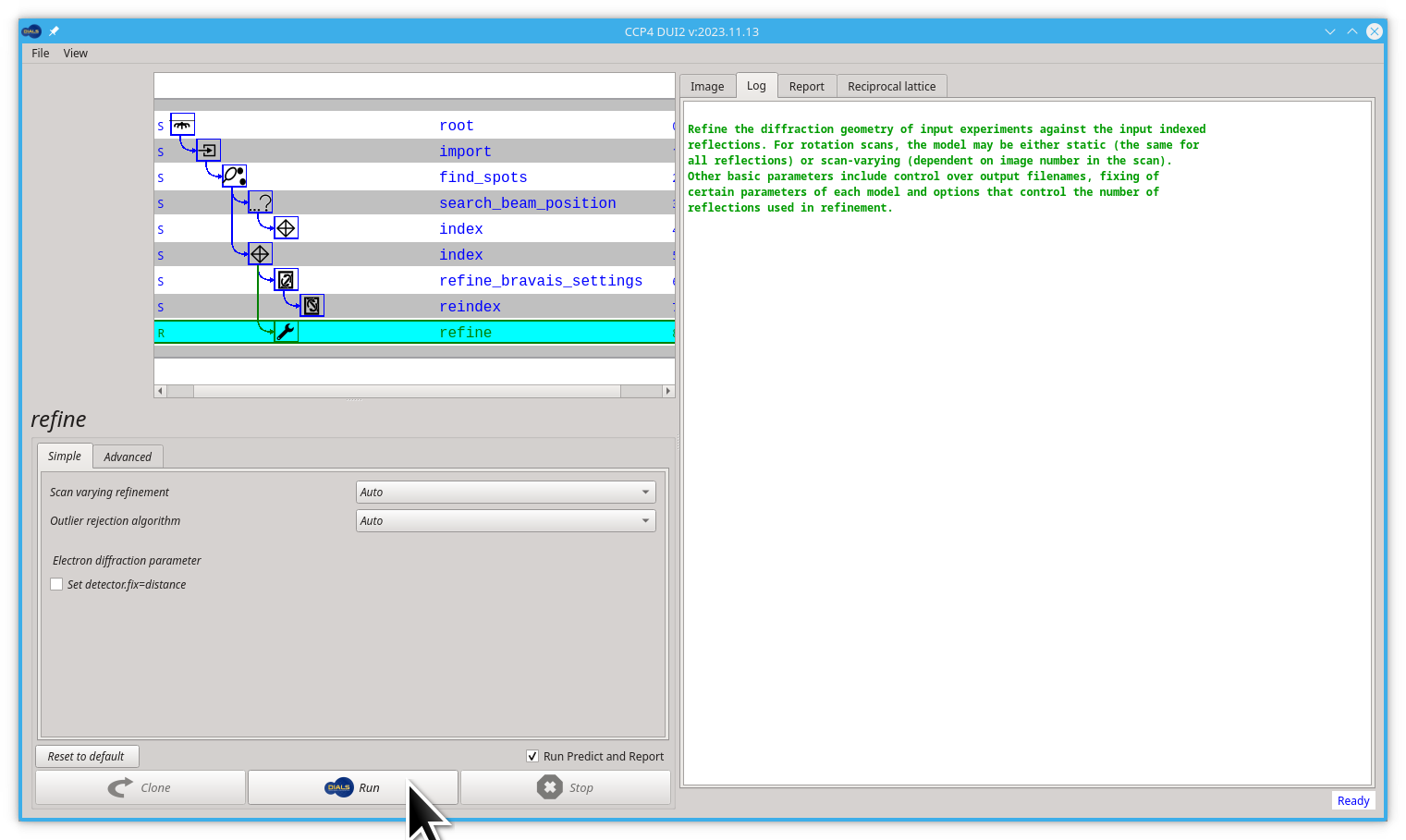
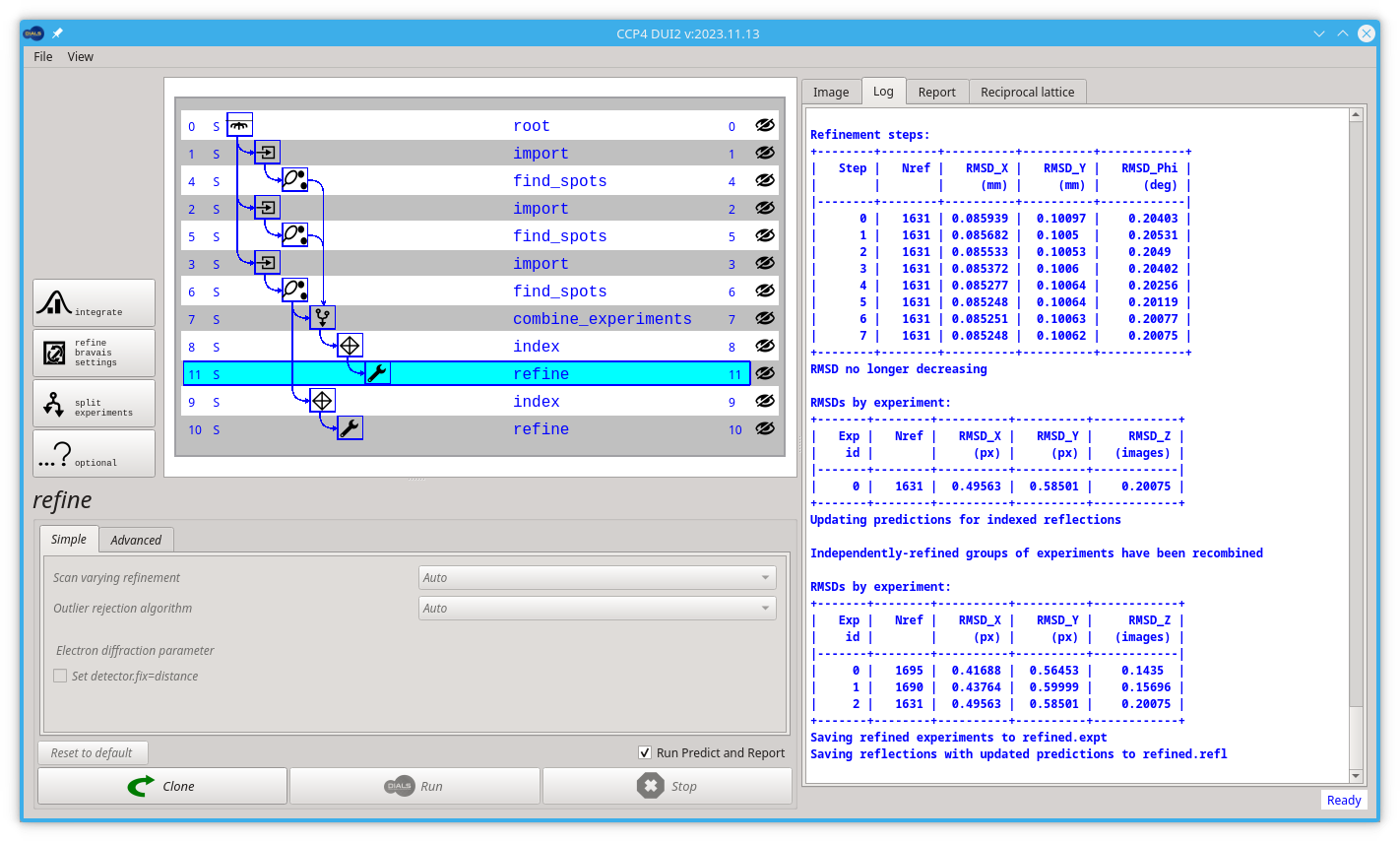
The model is already refined during indexing, but this is assuming that a single crystal model is appropriate for every image in the data set. In reality, there are usually small changes in the unit cell and crystal orientation throughout the experiment as the sample is rotated. dials.refine will first re-run refinement with a fixed unit cell and then perform scan-varying refinement. If you have indexed multiple sweeps earlier in processing (not covered in this tutorial), then the crystal models will be copied and split at this stage to allow per-crystal-per-scan models to be refined.

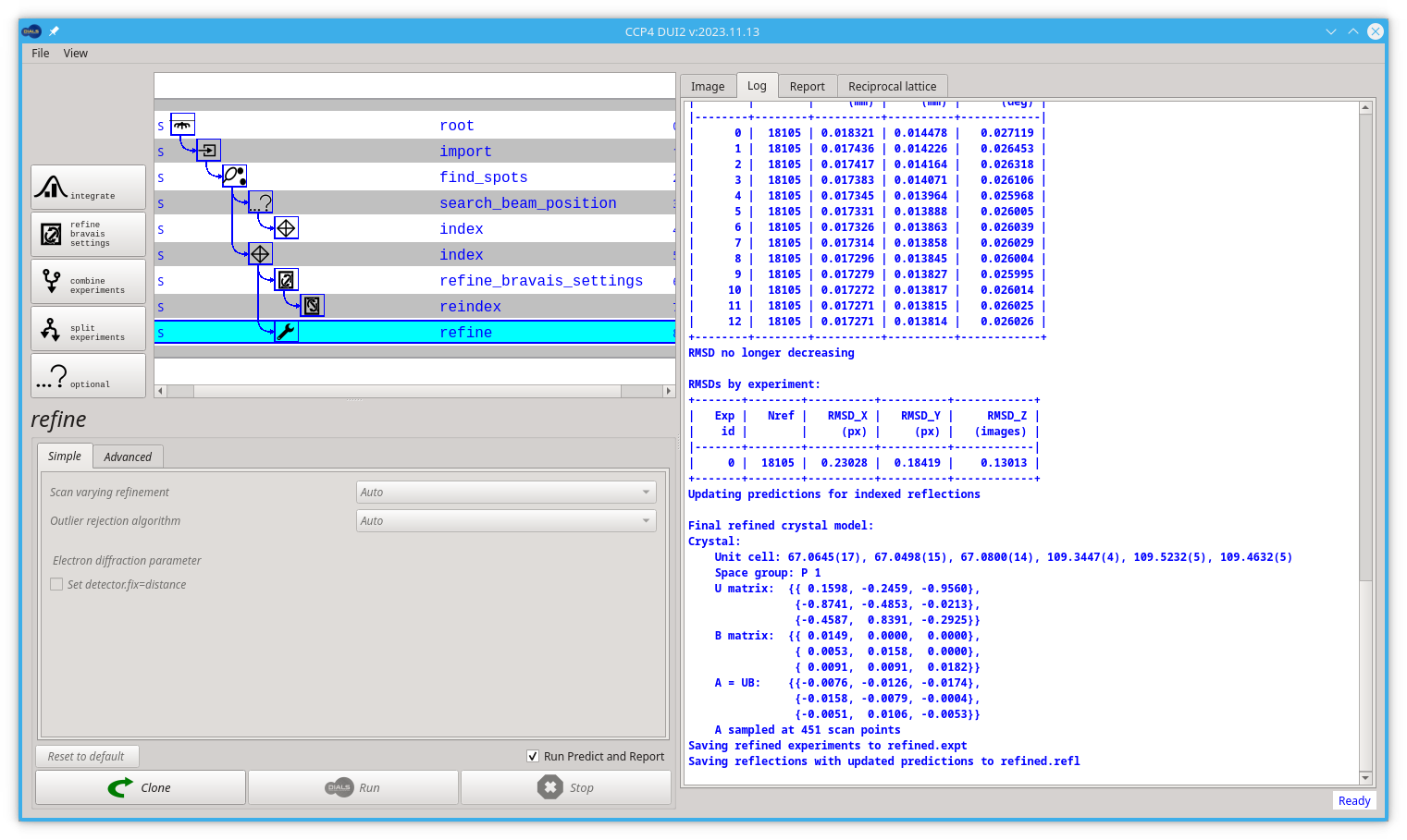
Without any options, the program will do something sensible. If you compare the R.M.S. deviations from the end of indexing with the end of refinement you should see a small improvement e.g.

RMSDs by experiment:
+-------+--------+----------+----------+------------+
|   Exp |   Nref |   RMSD_X |   RMSD_Y |     RMSD_Z |
|    id |        |     (px) |     (px) |   (images) |
|-------+--------+----------+----------+------------|
|     0 |   8999 |  0.25876 |  0.22032 |    0.18062 |
+-------+--------+----------+----------+------------+

to:

RMSDs by experiment:
+-------+--------+----------+----------+------------+
|   Exp |   Nref |   RMSD_X |   RMSD_Y |     RMSD_Z |
|    id |        |     (px) |     (px) |   (images) |
|-------+--------+----------+----------+------------|
|     0 |  18105 |  0.23028 |  0.18419 |    0.13013 |
+-------+--------+----------+----------+------------+

If you look at the output of dials.report at this stage, you should see small variations in the unit cell and sample orientation as the crystal is rotated. If these do not appear small, then it is likely that something has happened during data collection e.g. severe radiation damage.

Integration

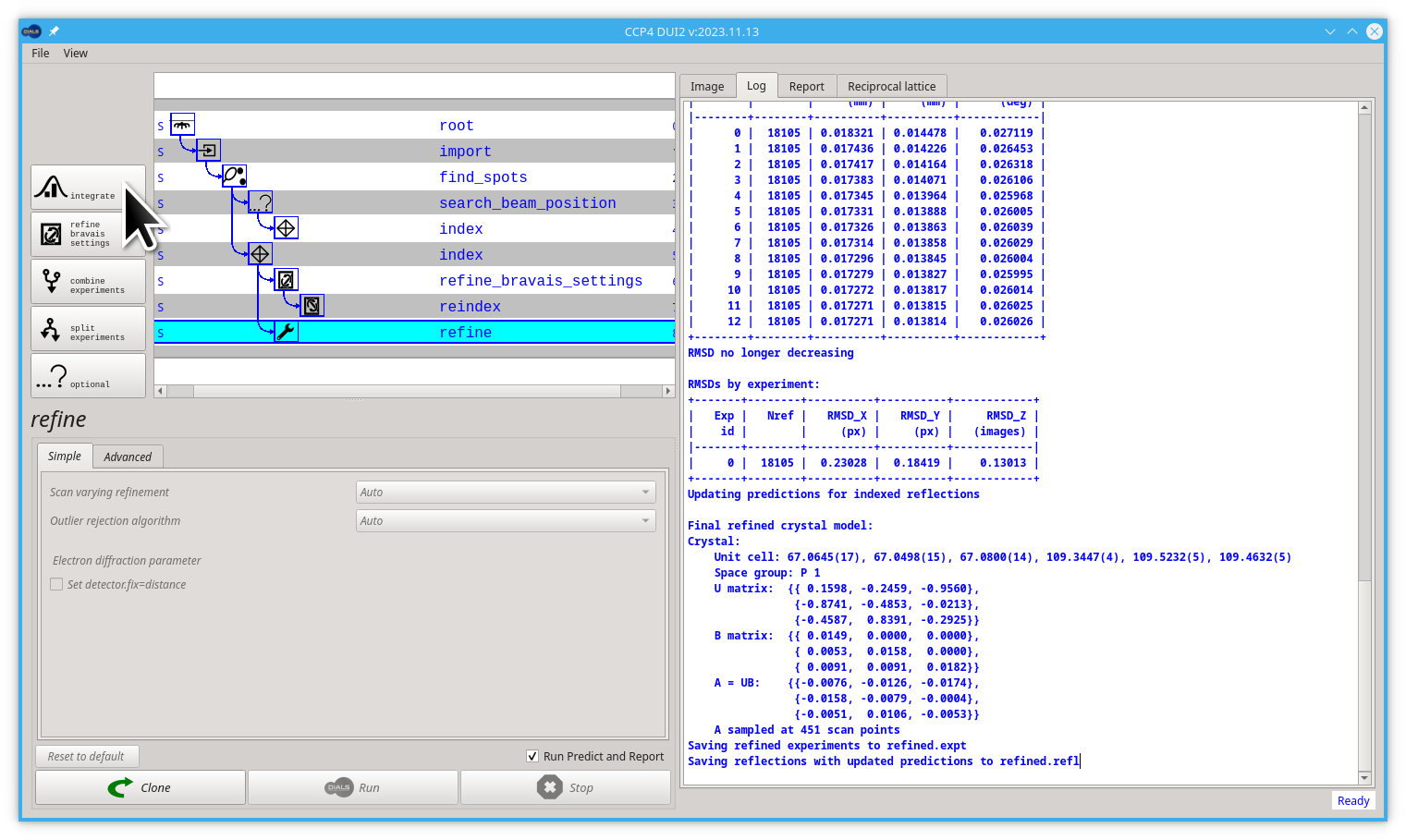
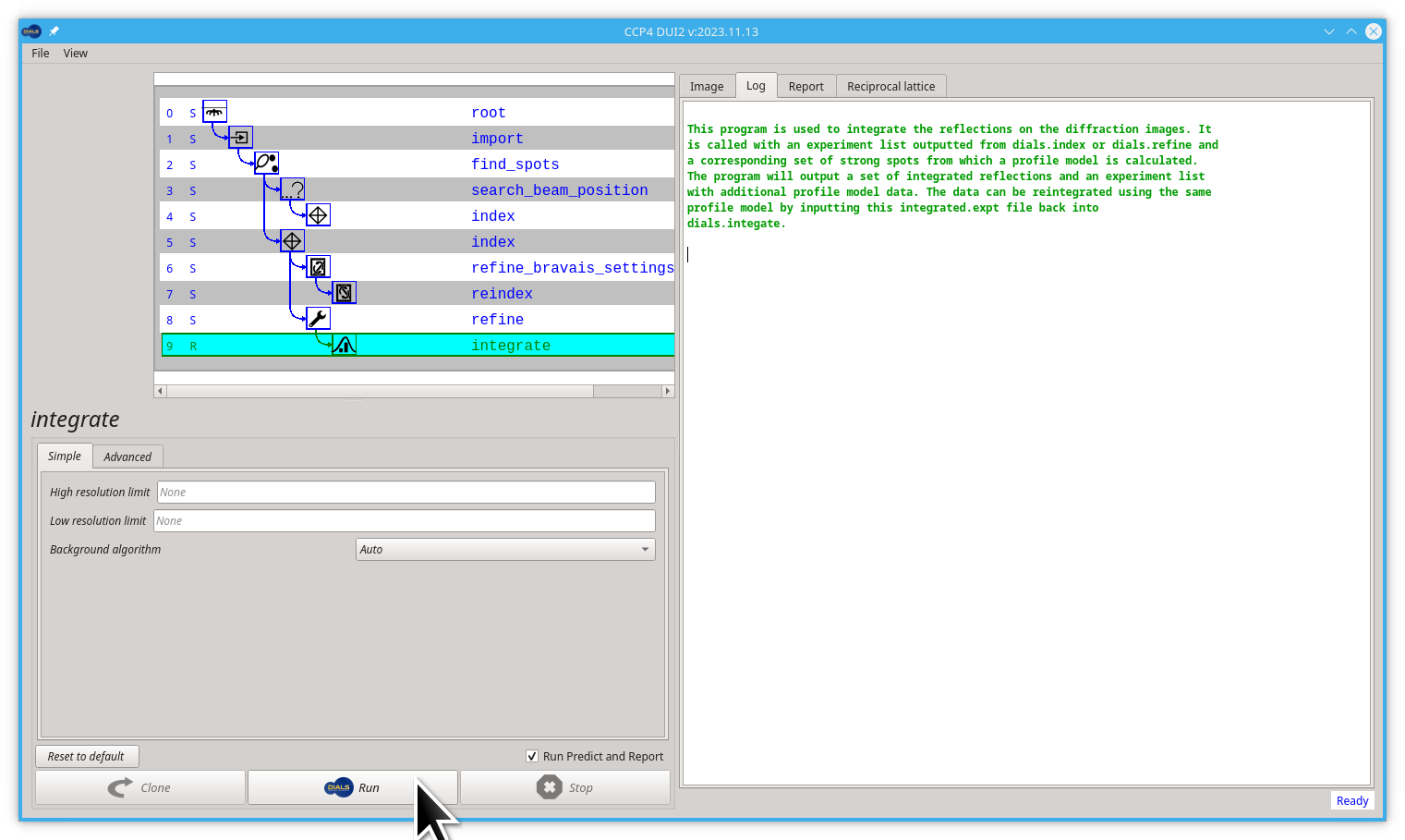
Once you have refined the model, the next step is to integrate the data. In effect this is using the refined model to calculate the positions where all of the reflections in the data set will be found and measure the background-subtracted intensities:

Let's start by creating the new node, click the Integrate button.

Now click on the Run button, to launch the dials.integrate command.

By default this will pass through the data twice, first looking at the shapes of the predicted spots to form a reference profile model, then passing through a second time to use this profile model to integrate the data, by being fit into the transformed pixel values. This is by far the most computationally expensive step in the processing of the data!

By default, all the processors in your computer are used unless we think this will exceed the memory available on the machine. At times, however, if you have a large unit cell and / or a large data set, you may find that processing on a desktop workstation is more appropriate than a laptop or other types of weaker hardware.

At this stage, if you know in advance that the data does not diffract to anything close to the edges of the detector, you can assign a resolution limit by adding prediction.d_min=1.8 (say) to define a 1.8 Å resolution limit but in general, this should not be necessary.

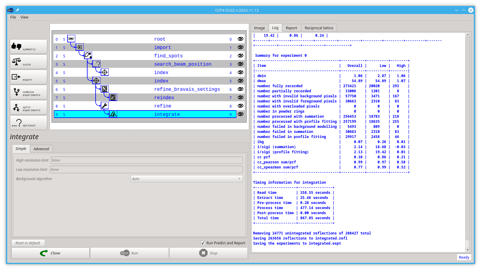
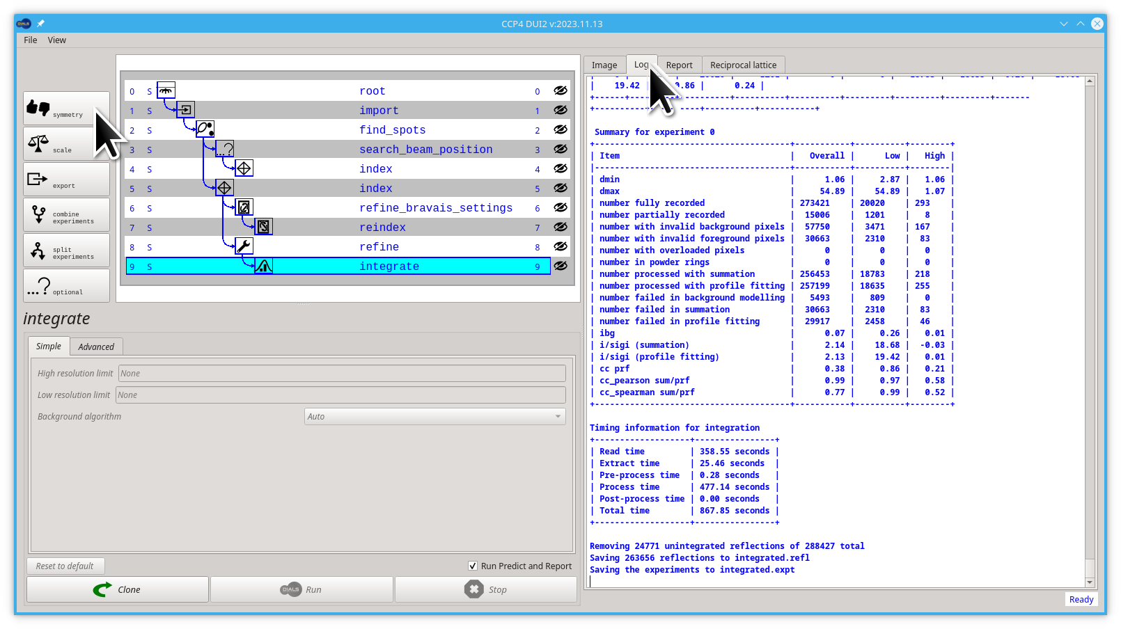
By the end of the integrate step, the output in the log tab of Dui2 should look like

We can have a look at the "boxes" that were used for integration, with the image viewer.

• Go back to the Image tab
• Pull down the Display info menu
• Select the Observation option back

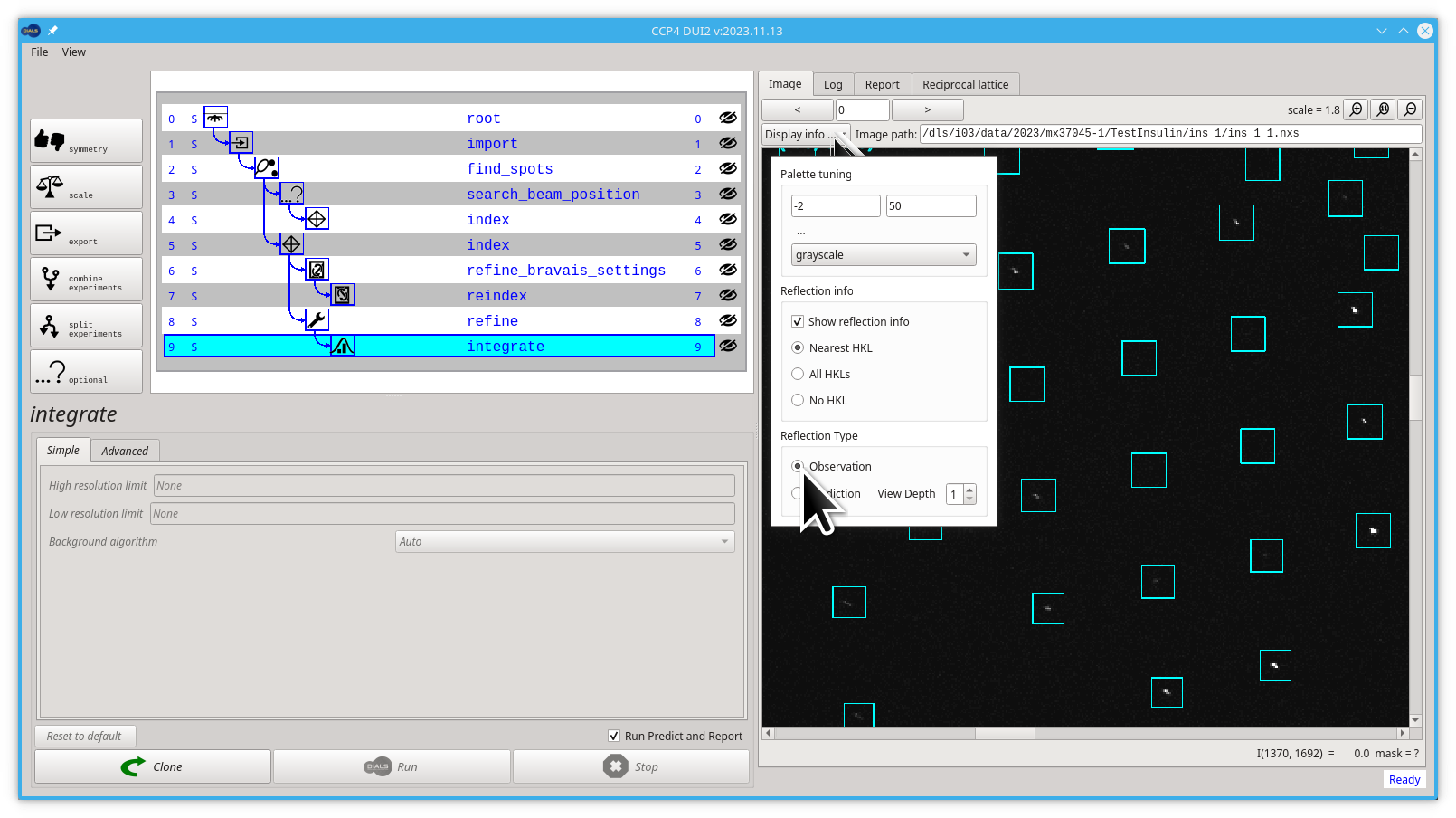
Here we can see that in every reflection that was integrated, DIALS uses a rectangular "box" that is bigger that the area where the reflection is. This extra area is used to estimate the background that needs to be subtracted from the "foreground" pixels to calculate the intensity.

Symmetry analysis

Before the data may be scaled, it is necessary that the crystal symmetry is known. If this was assigned correctly at indexing (e.g. space_group=I213) then you can proceed directly to scaling. In the majority of cases, however it will be unknown or not set at this point, so it needs to be assigned between integration and scaling. Even if the Bravais lattice was assigned earlier, the correct symmetry within that lattice is needed.

The symmetry analysis in DIALS takes the information from the spot positions and also the spot intensities. The former are used to effectively re-run dials.refine_bravais_settings to identify possible lattices and hence candidate symmetry operations, and the latter are used to assess the presence or absence of these symmetry operations. Once the operations are found, the crystal rotational symmetry is assigned by composing these operations into a putative space group. In addition, systematically absent reflections are also assessed to assign a best guess to translational elements of the symmetry. Though these are not needed for scaling, they may help with downstream analysis rather than you having to manually identify them.

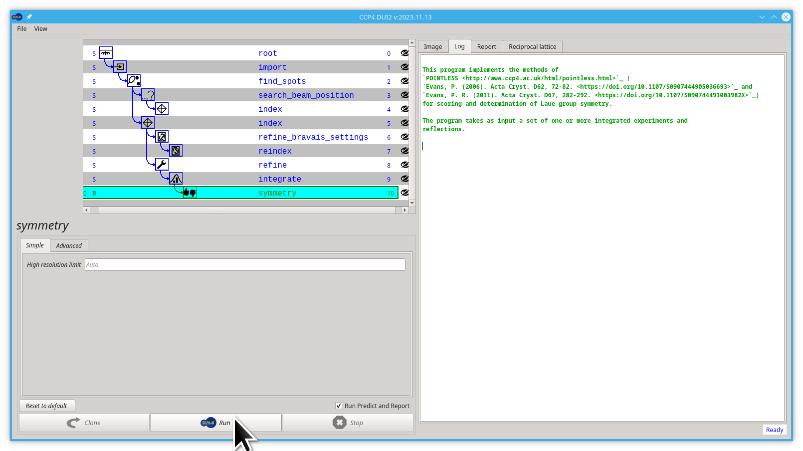
Let' run dials.symmetry , first put back the Log tab, then click the symmetry button.

Now click the Run button.

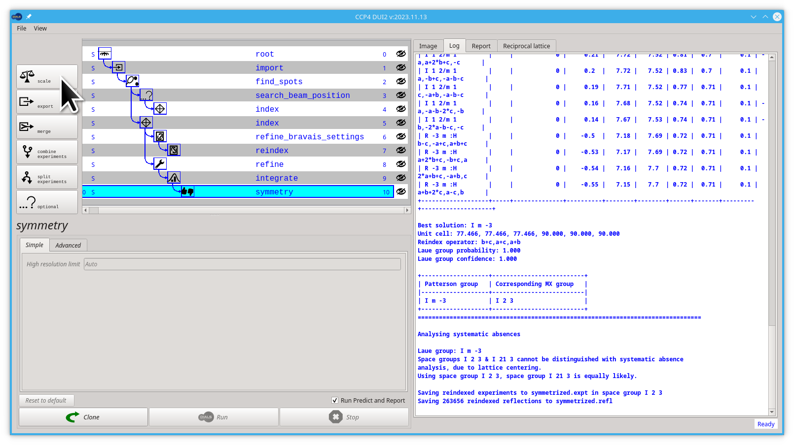
At this point it is important to note that the program is trying to identify all symmetry elements, and does not know that, let's say inversion centres, are not possible. For an oP lattice it will be testing for P/mmm symmetry which corresponds to P2?2?2? in standard MX.

The data in this tutorial gives an interesting output for this:

Scoring individual symmetry elements

+--------------+--------+------+-------+-----+---------------+
|   likelihood |   Z-CC |   CC |     N |     | Operator      |
|--------------+--------+------+-------+-----+---------------|
|        0.944 |   9.96 | 1    | 39920 | *** | 1 |(0, 0, 0)  |
|        0.154 |   4.35 | 0.43 | 70838 |     | 4 |(1, 1, 0)  |
|        0.158 |   4.43 | 0.44 | 35098 |     | 4 |(1, 0, 1)  |
|        0.161 |   4.48 | 0.45 | 57110 |     | 4 |(0, 1, 1)  |
|        0.943 |   9.93 | 0.99 | 46454 | *** | 3 |(1, 0, 0)  |
|        0.943 |   9.93 | 0.99 | 71108 | *** | 3 |(0, 1, 0)  |
|        0.943 |   9.95 | 0.99 | 50430 | *** | 3 |(0, 0, 1)  |
|        0.943 |   9.94 | 0.99 | 43104 | *** | 3 |(1, 1, 1)  |
|        0.943 |   9.94 | 0.99 | 30300 | *** | 2 |(1, 1, 0)  |
|        0.158 |   4.43 | 0.44 | 35202 |     | 2 |(-1, 1, 0) |
|        0.943 |   9.95 | 0.99 | 38900 | *** | 2 |(1, 0, 1)  |
|        0.163 |   4.53 | 0.45 | 28216 |     | 2 |(-1, 0, 1) |
|        0.944 |   9.95 | 1    | 30760 | *** | 2 |(0, 1, 1)  |
|        0.16  |   4.46 | 0.45 | 24160 |     | 2 |(0, -1, 1) |
|        0.154 |   4.35 | 0.43 | 37206 |     | 2 |(1, 1, 2)  |
|        0.161 |   4.49 | 0.45 | 27406 |     | 2 |(1, 2, 1)  |
|        0.151 |   4.29 | 0.43 | 31700 |     | 2 |(2, 1, 1)  |
+--------------+--------+------+-------+-----+---------------+

Here it is clear that there are some operations that have close to 100% CC. Others that are much lower, in particular the 4-fold rotations in the middle of the faces, are not present which means the crystal has a polar space group so care needs to be taken when combining data from multiple samples.

After finishing the symmetry step, Dui2 should look like this:

You may click the scale button to move to the scale step.

Scaling and Merging

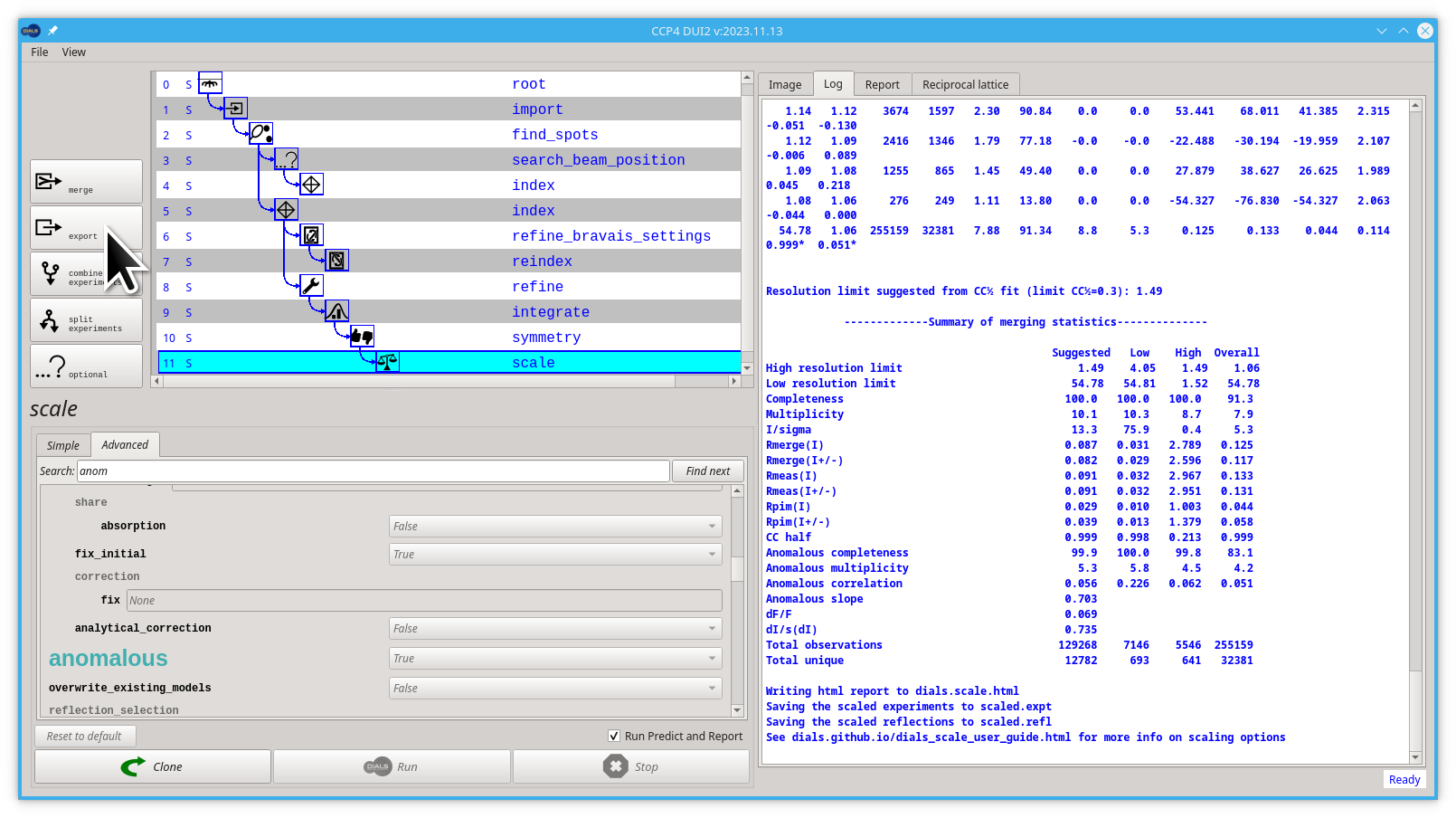
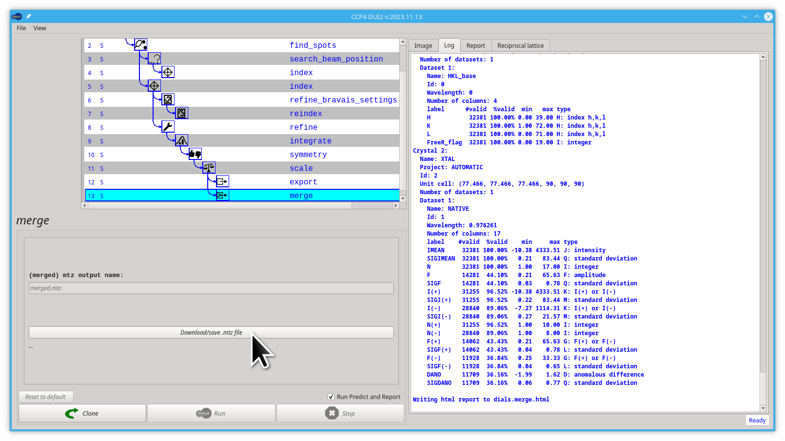
During the experiment, there are effects which alter the measured intensity of the reflections, not least radiation damage, changes to beam intensity or illuminated volume or absorption within the sample. The purpose of dials.scale, like all scaling programs, is to attempt to correct for these effects by using the fact that symmetry related reflections should share a common intensity. By default, no attempt is made to merge the reflections. This may be done independently in dials.merge but a table of merging statistics is printed at the end along with resolution recommendations.

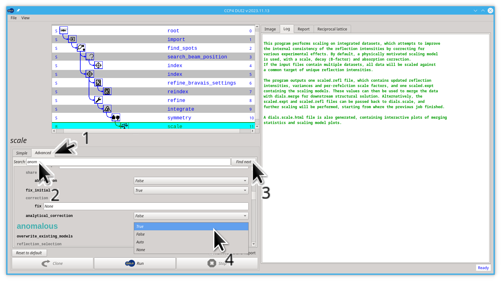
In the scale step, we are going to try one of the Advanced parameters(anomalous set to True). What we are going to do will be translated by Dui2 to the following command:

    dials.scale symmetrized.expt symmetrized.refl [anomalous=True]

Which will run with the defaults and allow for:

• modest radiation damage
• changes in overall intensity
• modest sample absorption

Let's edit this anomalous parameter:

• Click on the Advanced tab
• start typing "anomalous" on the Search box, you don't need to finish typing, "anom" is enough
• click the Find next button
• Pull down the menu next to the big, green "anomalous" label and select True

Now you can launch dials.scale by clicking the Run button.

The sample absorption parameter will most likely change. If you have a data set recorded from a sample containing a large amount of metal (not common in MX) or recorded at long wavelength (e.g., for sulphur SAD) it may be necessary to adjust the extent to which the absorption correction is constrained with

    absorption_level=(low|medium|high)

where setting low (the default) corresponds to ~ 1% absorption, medium to ~5% and high to ~ 25%. These are not absolute, instead more of a sense of what you may expect. Testing has indicated that setting it too high is unlikely to do any harm, but setting it too low can have a measurable impact on the quality of the data for phasing experiments. We are not touching the absorption_level parameter in this tutorial.

dials.scale generates a HTML report called dials.scale.html which includes a lot of information on how the models look, as well as regions of the data which agree well and poorly. From a practical perspective, this is the point where you really know about the final quality of the data. This HTML file is used by Dui2 to replace the automatically generated one after the scale step, it can be seen in the Report step.

Merging or Exporting

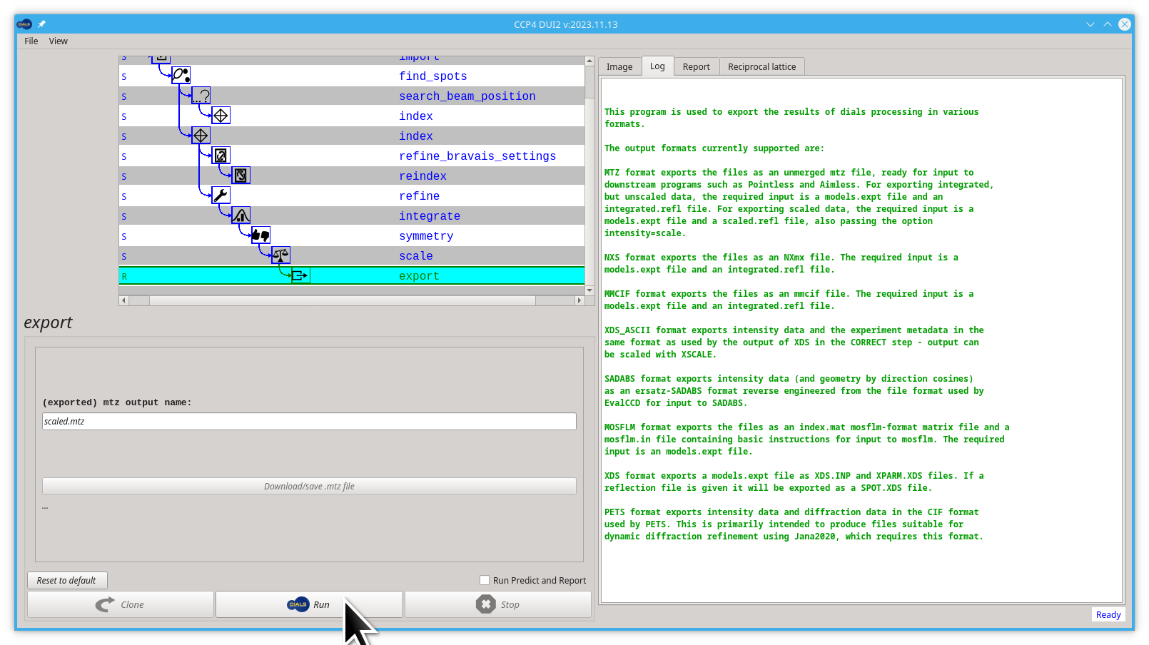
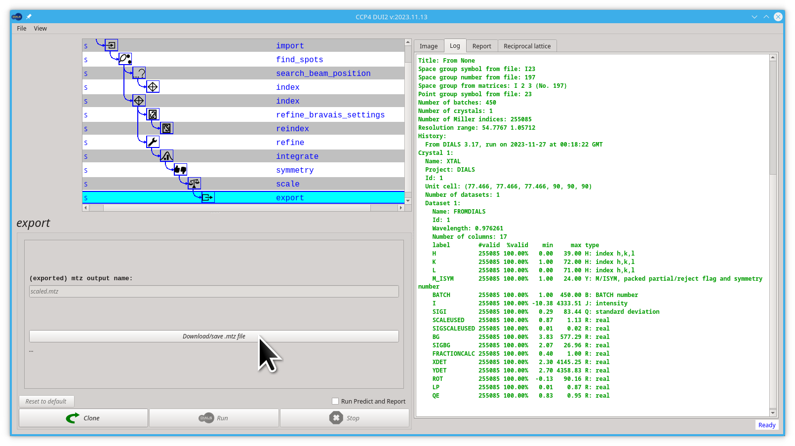
Most downstream software depends on a scaled and merged data set for, let's say molecular replacement, so at the end of processing you can run

    dials.export

to simply export the scaled reflections in the MTZ format or

    dials.merge

which will output a scaled and merged MTZ file.

After the next two step is important to remember where are you saving your .mtz files as they will be needed for processing your data further.

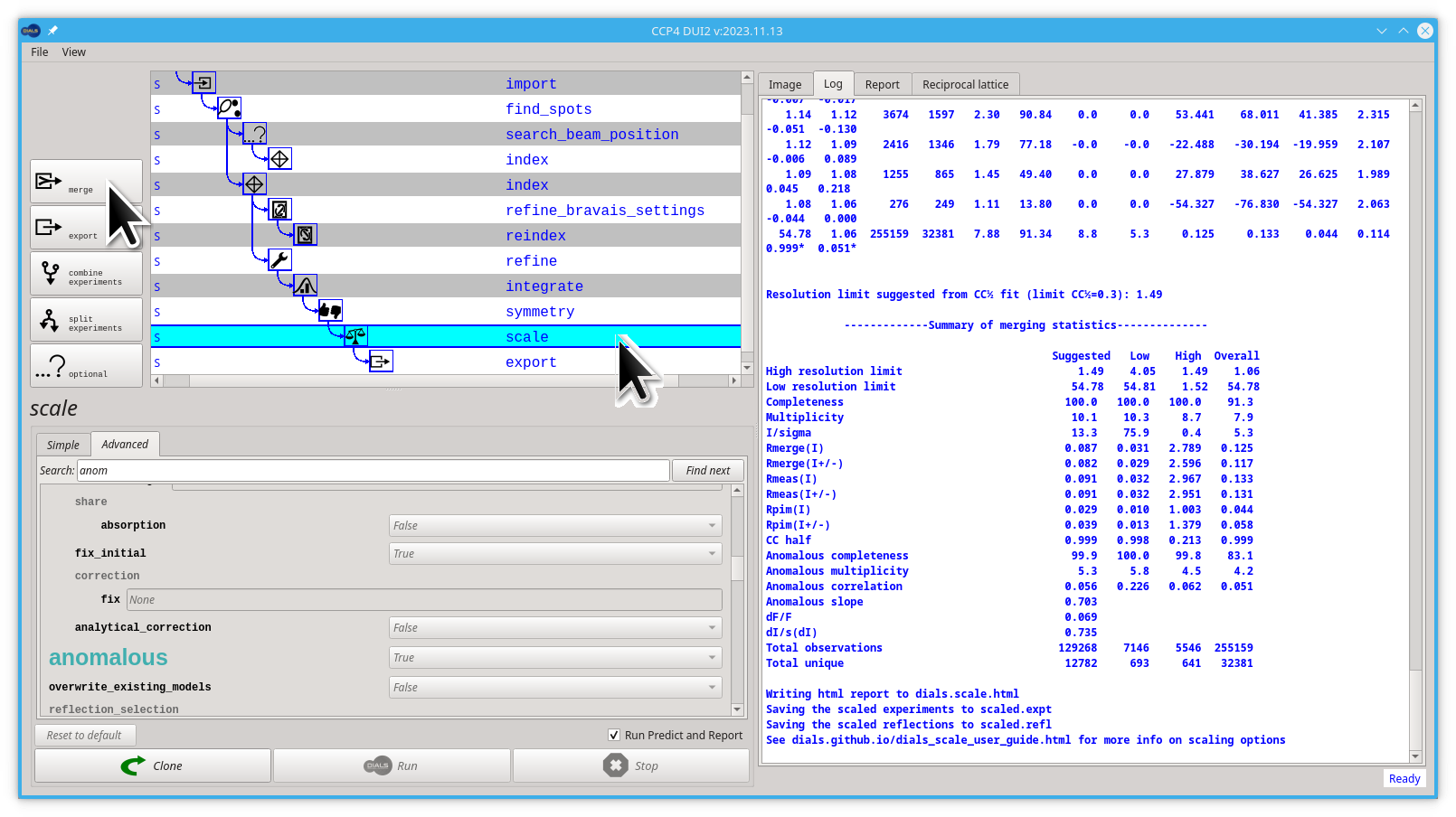
Let's do both, export and merge:

• First click the export button to create the new export node

• Then click the Run button

• Now you can save the scaled.mtz file by clicking the Download/save mtz file button

If you want to merge your results you should:

• Go back to the scale node

• Click the merge button

• Click the Run button

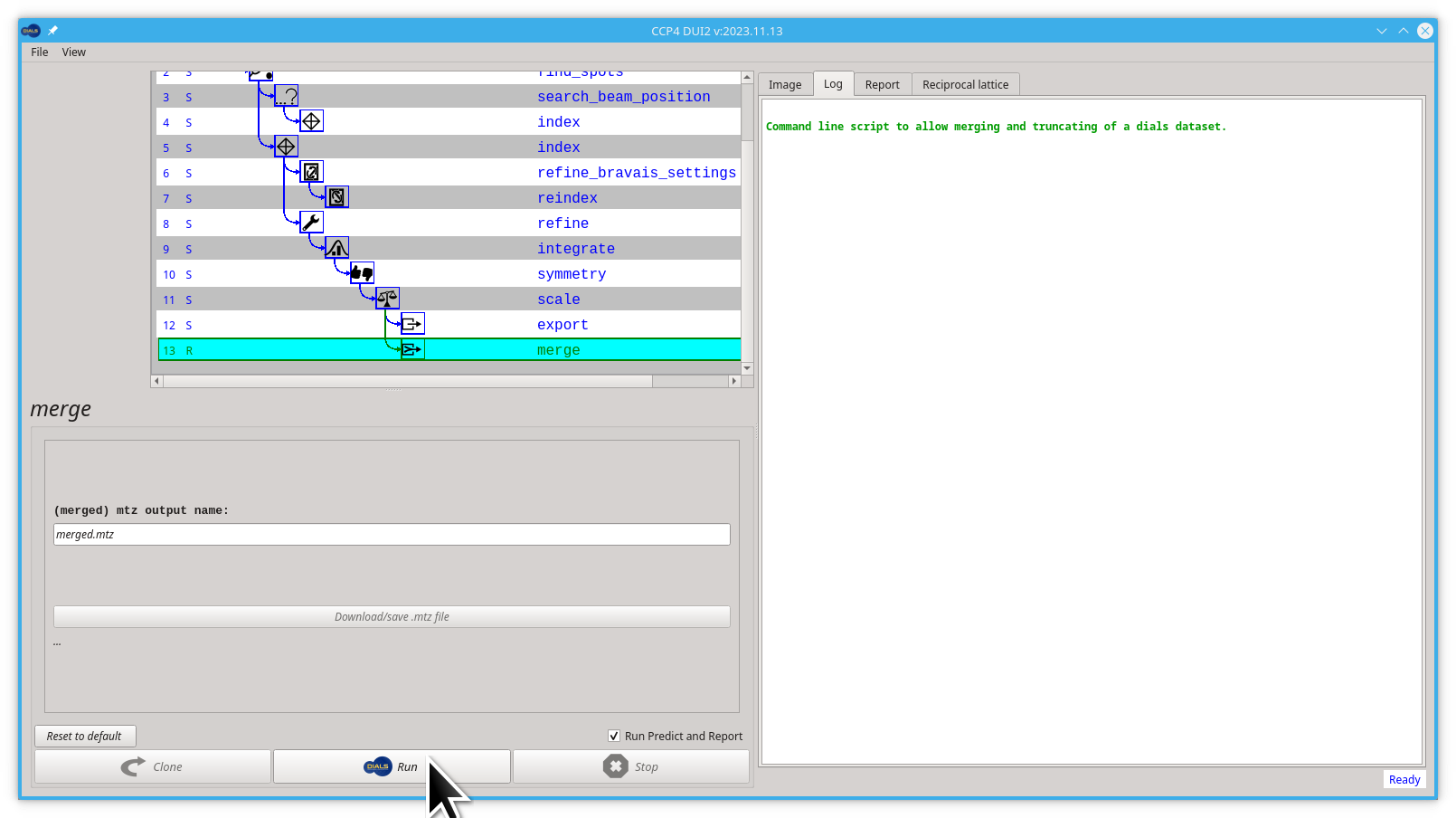
• Now you can save the merged.mtz file by clicking the Download/save mtz file button

If you remember where you saved it. Your .mtz file is ready for further processing.

Thanks to Graeme Winter for writing the command line tutorial of which this one is based on.