Phodo의 포토가이드 만들기 서비스를 지원하기 위해 적용한이미지 세그멘테이션 모델
- Deep Learning
- Computer Vision
- CNN
- Yolov5
- Mask RCNN
- Pytorch
- Tensorflow
- OpenCV
- Google Colab
사진의 인물(사람)의 외곽선만을 추출하기 위해 이미지 세그멘테이션 모델을 사용했습니다.
초반에는 Mask RCNN 을 사용했으나 외곽선 추출이 깔끔하지 못하여 더 높은 성능을 보이는 yoloyv5 모델을 사용했습니다.
인물의 외곽선만을 추출하기 위해 yolov5-utils-plots.py 코드를 수정했습니다. 코드 실행을 통해 다음과 같은 데이터를 지정된 폴더에 저장합니다
- 원본 이미지
- 외곽선에 데이터 (.json) -> 선만 추출
- 조정된 이미지의 사이즈 데이터 (.json)
- 인물 mask 이미지 -> 인물만 검정색 mask로 표시
for index, mask in enumerate(masks):
          # person : 0 만 추출
          if(labels[index] == 0):
            #padded_mask = np.zeros((mask.shape[0] + 2, mask.shape[1] + 2), dtype=np.uint8)
            #padded_mask[1:-1, 1:-1] = mask
            mask = scale_image(mask.shape, mask, self.im.shape)
            h,w = mask.shape[:2]
            length_dic["width"] = w
            length_dic["height"] = h

            contours, _ = cv2.findContours(mask.astype(np.uint8), cv2.RETR_EXTERNAL, cv2.CHAIN_APPROX_NONE)
            cv2.drawContours(black_contour_img, contours, -1, (255,255,255), 4) #contour_img


            tmp_list = []

            #json 파일로 contours를 인덱싱하여 저장합니다.
            print(len(contours[0]))
            for i in range(0,len(contours[0])):
              point_dic = {}
              point_dic["x"] = np.double(contours[0][i][0][0])
              point_dic["y"] = np.double(contours[0][i][0][1])
              tmp_list.append(point_dic)

            json_contour_data[str(count)] = tmp_list
            count = count + 1

        with open('/gdrive/My Drive/PHODO/Segmentation Model/Yolo_custom/yolov5/trevi_length_dic.json','w') as f:
            json.dump(length_dic, f)

        with open('/gdrive/My Drive/PHODO/Segmentation Model/Yolo_custom/yolov5/trevi_contour_data.json','w') as f:
          json.dump(json_contour_data, f)

        black_contour_img = cv2.cvtColor(black_contour_img, cv2.COLOR_BGR2RGB)
현재 yolov5 오픈소스의 출력값 코드를 변형하는 방식으로 원하는 데이터를 얻어내고 있습니다.
또한 google colab 에서 실험한 코드를 앱에 적용시키는 부분을 계속해서 고민하고 있습니다.
다음과 같은 3가지 방법을 시도할 계획입니다.
- 앱 자체에 모델을 내장 (모델을 SDK 로 만들어 통합 빌드)
- 안드로이드에서 colab에 접근해 연동
- server에 모델을 올리고 안드로이드은 서버에 요청
.
├── Mask_RCNN-TF2
├── Yolo (origin source)
└── Yolo_custom (custom source, actually used in the app)
    └── yolov5
        ├── calssify
        ├── data
        ├── models
        ├── segment
        └── utils
YOLOv5 🚀 is the world's most loved vision AI, representing Ultralytics open-source research into future vision AI methods, incorporating lessons learned and best practices evolved over thousands of hours of research and development.
We hope that the resources here will help you get the most out of YOLOv5. Please browse the YOLOv5 Docs for details, raise an issue on GitHub for support, and join our Discord community for questions and discussions!
To request an Enterprise License please complete the form at Ultralytics Licensing.
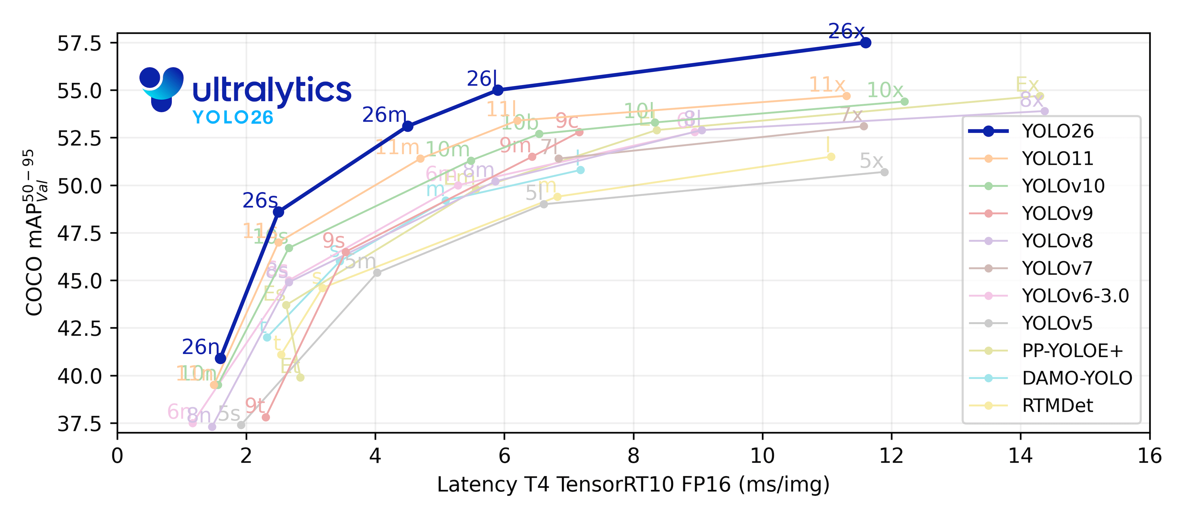
We are thrilled to announce the launch of Ultralytics YOLOv8 🚀, our NEW cutting-edge, state-of-the-art (SOTA) model released at https://github.com/ultralytics/ultralytics. YOLOv8 is designed to be fast, accurate, and easy to use, making it an excellent choice for a wide range of object detection, image segmentation and image classification tasks.
See the YOLOv8 Docs for details and get started with:
pip install ultralyticsSee the YOLOv5 Docs for full documentation on training, testing and deployment. See below for quickstart examples.
Install
Clone repo and install requirements.txt in a Python>=3.7.0 environment, including PyTorch>=1.7.
git clone https://github.com/ultralytics/yolov5  # clone
cd yolov5
pip install -r requirements.txt  # install
Inference
YOLOv5 PyTorch Hub inference. Models download automatically from the latest YOLOv5 release.
import torch

# Model
model = torch.hub.load("ultralytics/yolov5", "yolov5s")  # or yolov5n - yolov5x6, custom

# Images
img = "https://ultralytics.com/images/zidane.jpg"  # or file, Path, PIL, OpenCV, numpy, list

# Inference
results = model(img)

# Results
results.print()  # or .show(), .save(), .crop(), .pandas(), etc.
Inference with detect.py
detect.py runs inference on a variety of sources, downloading models automatically from
the latest YOLOv5 release and saving results to runs/detect.
python detect.py --weights yolov5s.pt --source 0                               # webcam
                                               img.jpg                         # image
                                               vid.mp4                         # video
                                               screen                          # screenshot
                                               path/                           # directory
                                               list.txt                        # list of images
                                               list.streams                    # list of streams
                                               'path/*.jpg'                    # glob
                                               'https://youtu.be/Zgi9g1ksQHc'  # YouTube
                                               'rtsp://example.com/media.mp4'  # RTSP, RTMP, HTTP stream
Training
The commands below reproduce YOLOv5 COCO
results. Models
and datasets download automatically from the latest
YOLOv5 release. Training times for YOLOv5n/s/m/l/x are
1/2/4/6/8 days on a V100 GPU (Multi-GPU times faster). Use the
largest --batch-size possible, or pass --batch-size -1 for
YOLOv5 AutoBatch. Batch sizes shown for V100-16GB.
python train.py --data coco.yaml --epochs 300 --weights '' --cfg yolov5n.yaml  --batch-size 128
                                                                 yolov5s                    64
                                                                 yolov5m                    40
                                                                 yolov5l                    24
                                                                 yolov5x                    16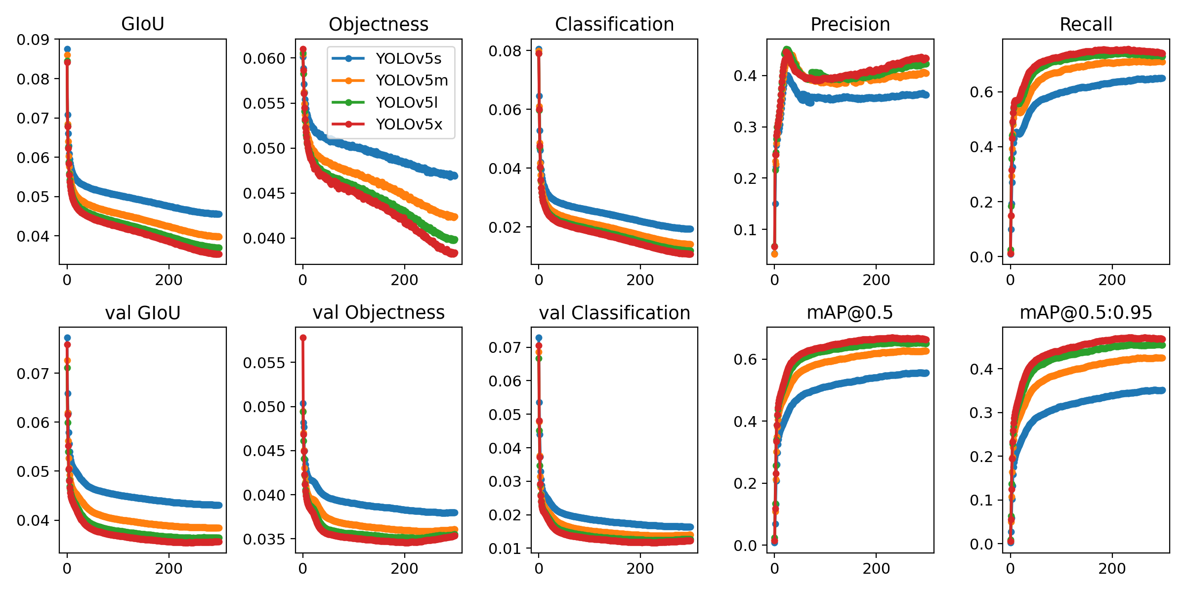
Tutorials
- Train Custom Data 🚀 RECOMMENDED
- Tips for Best Training Results ☘️
- Multi-GPU Training
- PyTorch Hub 🌟 NEW
- TFLite, ONNX, CoreML, TensorRT Export 🚀
- NVIDIA Jetson platform Deployment 🌟 NEW
- Test-Time Augmentation (TTA)
- Model Ensembling
- Model Pruning/Sparsity
- Hyperparameter Evolution
- Transfer Learning with Frozen Layers
- Architecture Summary 🌟 NEW
- Roboflow for Datasets, Labeling, and Active Learning
- ClearML Logging 🌟 NEW
- YOLOv5 with Neural Magic's Deepsparse 🌟 NEW
- Comet Logging 🌟 NEW

| Roboflow | ClearML ⭐ NEW | Comet ⭐ NEW | Neural Magic ⭐ NEW |
|---|---|---|---|
| Label and export your custom datasets directly to YOLOv5 for training with Roboflow | Automatically track, visualize and even remotely train YOLOv5 using ClearML (open-source!) | Free forever, Comet lets you save YOLOv5 models, resume training, and interactively visualise and debug predictions | Run YOLOv5 inference up to 6x faster with Neural Magic DeepSparse |
Experience seamless AI with Ultralytics HUB ⭐, the all-in-one solution for data visualization, YOLOv5 and YOLOv8 🚀 model training and deployment, without any coding. Transform images into actionable insights and bring your AI visions to life with ease using our cutting-edge platform and user-friendly Ultralytics App. Start your journey for Free now!

YOLOv5 has been designed to be super easy to get started and simple to learn. We prioritize real-world results.
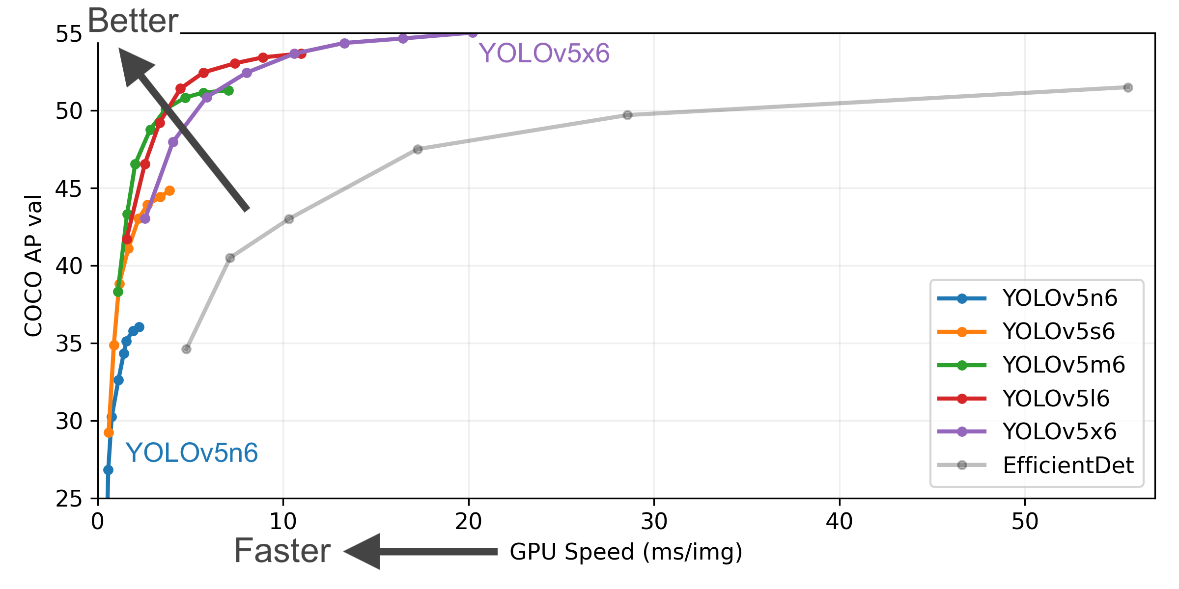
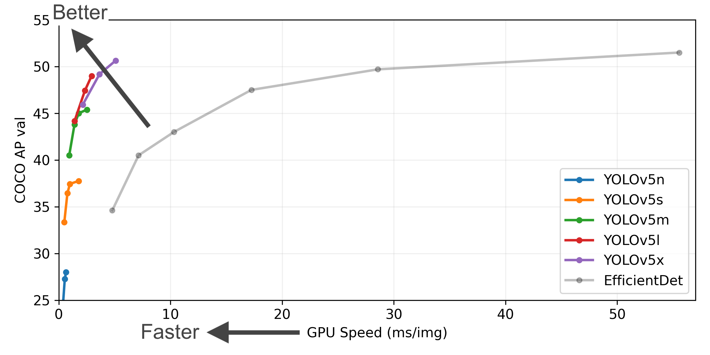
Figure Notes
- COCO AP val denotes [email protected]:0.95 metric measured on the 5000-image COCO val2017 dataset over various inference sizes from 256 to 1536.
- GPU Speed measures average inference time per image on COCO val2017 dataset using a AWS p3.2xlarge V100 instance at batch-size 32.
- EfficientDet data from google/automl at batch size 8.
- Reproduce by
python val.py --task study --data coco.yaml --iou 0.7 --weights yolov5n6.pt yolov5s6.pt yolov5m6.pt yolov5l6.pt yolov5x6.pt
| Model | size (pixels) |
mAPval 50-95 |
mAPval 50 |
Speed CPU b1 (ms) |
Speed V100 b1 (ms) |
Speed V100 b32 (ms) |
params (M) |
FLOPs @640 (B) |
|---|---|---|---|---|---|---|---|---|
| YOLOv5n | 640 | 28.0 | 45.7 | 45 | 6.3 | 0.6 | 1.9 | 4.5 |
| YOLOv5s | 640 | 37.4 | 56.8 | 98 | 6.4 | 0.9 | 7.2 | 16.5 |
| YOLOv5m | 640 | 45.4 | 64.1 | 224 | 8.2 | 1.7 | 21.2 | 49.0 |
| YOLOv5l | 640 | 49.0 | 67.3 | 430 | 10.1 | 2.7 | 46.5 | 109.1 |
| YOLOv5x | 640 | 50.7 | 68.9 | 766 | 12.1 | 4.8 | 86.7 | 205.7 |
| YOLOv5n6 | 1280 | 36.0 | 54.4 | 153 | 8.1 | 2.1 | 3.2 | 4.6 |
| YOLOv5s6 | 1280 | 44.8 | 63.7 | 385 | 8.2 | 3.6 | 12.6 | 16.8 |
| YOLOv5m6 | 1280 | 51.3 | 69.3 | 887 | 11.1 | 6.8 | 35.7 | 50.0 |
| YOLOv5l6 | 1280 | 53.7 | 71.3 | 1784 | 15.8 | 10.5 | 76.8 | 111.4 |
| YOLOv5x6 + TTA |
1280 1536 |
55.0 55.8 |
72.7 72.7 |
3136 - |
26.2 - |
19.4 - |
140.7 - |
209.8 - |
Table Notes
- All checkpoints are trained to 300 epochs with default settings. Nano and Small models use hyp.scratch-low.yaml hyps, all others use hyp.scratch-high.yaml.
- mAPval values are for single-model single-scale on COCO val2017 dataset.
Reproduce bypython val.py --data coco.yaml --img 640 --conf 0.001 --iou 0.65 - Speed averaged over COCO val images using a AWS p3.2xlarge instance. NMS times (~1 ms/img) not included.
Reproduce bypython val.py --data coco.yaml --img 640 --task speed --batch 1 - TTA Test Time Augmentation includes reflection and scale augmentations.
Reproduce bypython val.py --data coco.yaml --img 1536 --iou 0.7 --augment
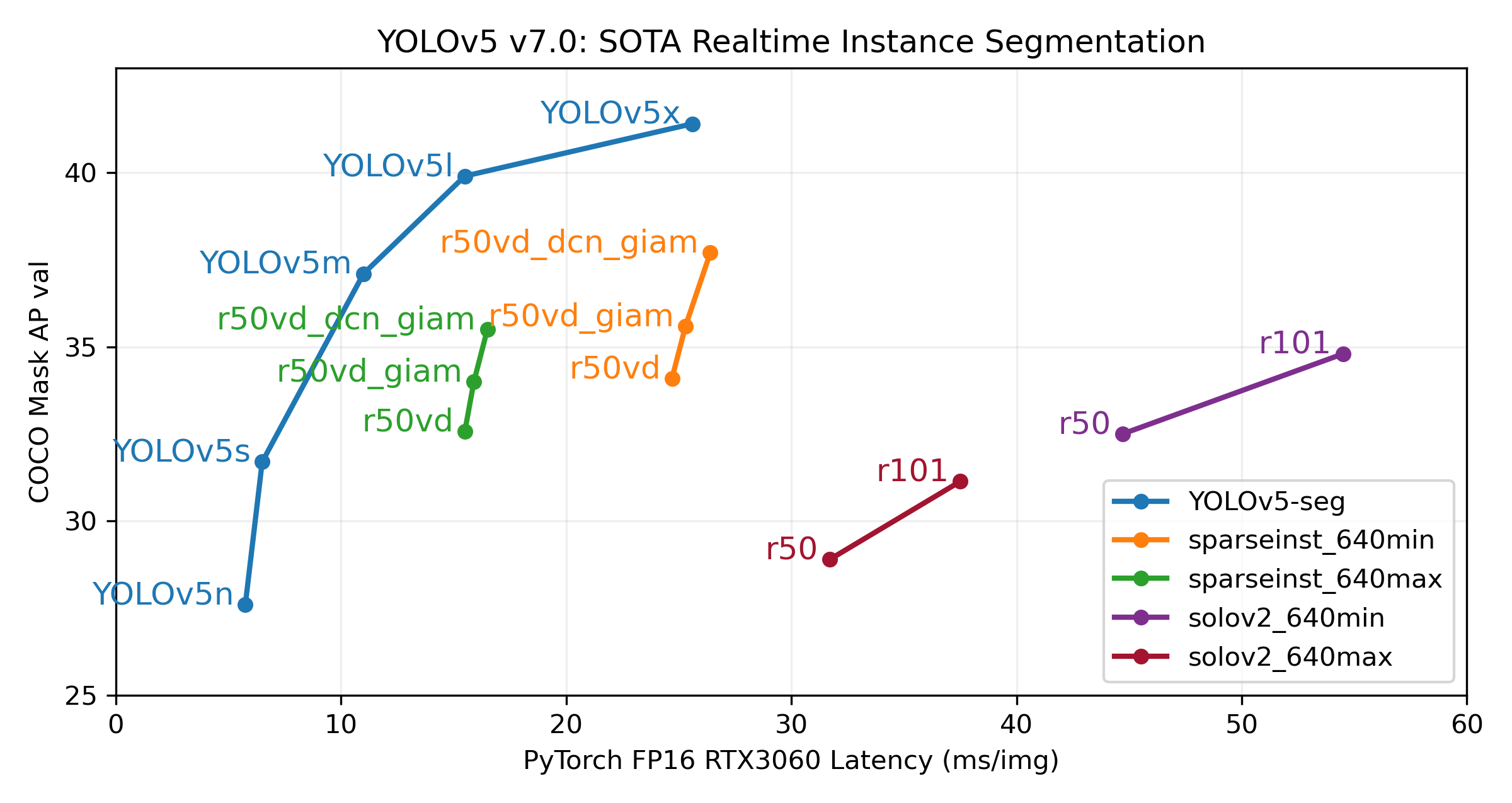
Our new YOLOv5 release v7.0 instance segmentation models are the fastest and most accurate in the world, beating all current SOTA benchmarks. We've made them super simple to train, validate and deploy. See full details in our Release Notes and visit our YOLOv5 Segmentation Colab Notebook for quickstart tutorials.
Segmentation Checkpoints
We trained YOLOv5 segmentations models on COCO for 300 epochs at image size 640 using A100 GPUs. We exported all models to ONNX FP32 for CPU speed tests and to TensorRT FP16 for GPU speed tests. We ran all speed tests on Google Colab Pro notebooks for easy reproducibility.
| Model | size (pixels) |
mAPbox 50-95 |
mAPmask 50-95 |
Train time 300 epochs A100 (hours) |
Speed ONNX CPU (ms) |
Speed TRT A100 (ms) |
params (M) |
FLOPs @640 (B) |
|---|---|---|---|---|---|---|---|---|
| YOLOv5n-seg | 640 | 27.6 | 23.4 | 80:17 | 62.7 | 1.2 | 2.0 | 7.1 |
| YOLOv5s-seg | 640 | 37.6 | 31.7 | 88:16 | 173.3 | 1.4 | 7.6 | 26.4 |
| YOLOv5m-seg | 640 | 45.0 | 37.1 | 108:36 | 427.0 | 2.2 | 22.0 | 70.8 |
| YOLOv5l-seg | 640 | 49.0 | 39.9 | 66:43 (2x) | 857.4 | 2.9 | 47.9 | 147.7 |
| YOLOv5x-seg | 640 | 50.7 | 41.4 | 62:56 (3x) | 1579.2 | 4.5 | 88.8 | 265.7 |
- All checkpoints are trained to 300 epochs with SGD optimizer with
lr0=0.01andweight_decay=5e-5at image size 640 and all default settings.
Runs logged to https://wandb.ai/glenn-jocher/YOLOv5_v70_official - Accuracy values are for single-model single-scale on COCO dataset.
Reproduce bypython segment/val.py --data coco.yaml --weights yolov5s-seg.pt - Speed averaged over 100 inference images using a Colab Pro A100 High-RAM instance. Values indicate inference speed only (NMS adds about 1ms per image).
Reproduce bypython segment/val.py --data coco.yaml --weights yolov5s-seg.pt --batch 1 - Export to ONNX at FP32 and TensorRT at FP16 done with
export.py.
Reproduce bypython export.py --weights yolov5s-seg.pt --include engine --device 0 --half
Segmentation Usage Examples 
YOLOv5 segmentation training supports auto-download COCO128-seg segmentation dataset with --data coco128-seg.yaml argument and manual download of COCO-segments dataset with bash data/scripts/get_coco.sh --train --val --segments and then python train.py --data coco.yaml.
# Single-GPU
python segment/train.py --data coco128-seg.yaml --weights yolov5s-seg.pt --img 640

# Multi-GPU DDP
python -m torch.distributed.run --nproc_per_node 4 --master_port 1 segment/train.py --data coco128-seg.yaml --weights yolov5s-seg.pt --img 640 --device 0,1,2,3Validate YOLOv5s-seg mask mAP on COCO dataset:
bash data/scripts/get_coco.sh --val --segments  # download COCO val segments split (780MB, 5000 images)
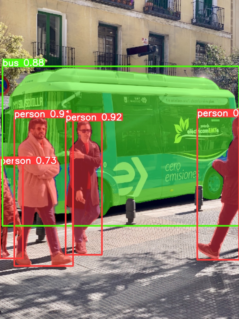
python segment/val.py --weights yolov5s-seg.pt --data coco.yaml --img 640 # validateUse pretrained YOLOv5m-seg.pt to predict bus.jpg:
python segment/predict.py --weights yolov5m-seg.pt --source data/images/bus.jpgmodel = torch.hub.load(
"ultralytics/yolov5", "custom", "yolov5m-seg.pt"
) # load from PyTorch Hub (WARNING: inference not yet supported)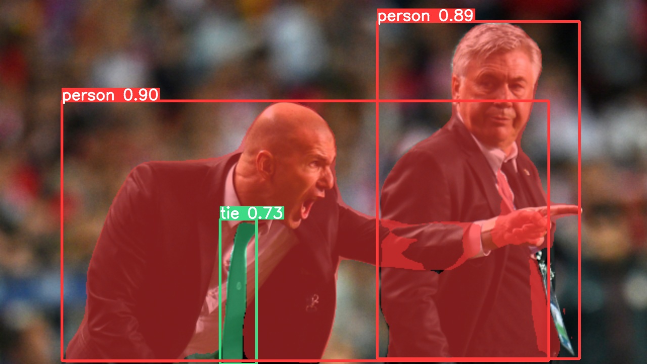 |
 |
|---|
Export YOLOv5s-seg model to ONNX and TensorRT:
python export.py --weights yolov5s-seg.pt --include onnx engine --img 640 --device 0YOLOv5 release v6.2 brings support for classification model training, validation and deployment! See full details in our Release Notes and visit our YOLOv5 Classification Colab Notebook for quickstart tutorials.
Classification Checkpoints
We trained YOLOv5-cls classification models on ImageNet for 90 epochs using a 4xA100 instance, and we trained ResNet and EfficientNet models alongside with the same default training settings to compare. We exported all models to ONNX FP32 for CPU speed tests and to TensorRT FP16 for GPU speed tests. We ran all speed tests on Google Colab Pro for easy reproducibility.
| Model | size (pixels) |
acc top1 |
acc top5 |
Training 90 epochs 4xA100 (hours) |
Speed ONNX CPU (ms) |
Speed TensorRT V100 (ms) |
params (M) |
FLOPs @224 (B) |
|---|---|---|---|---|---|---|---|---|
| YOLOv5n-cls | 224 | 64.6 | 85.4 | 7:59 | 3.3 | 0.5 | 2.5 | 0.5 |
| YOLOv5s-cls | 224 | 71.5 | 90.2 | 8:09 | 6.6 | 0.6 | 5.4 | 1.4 |
| YOLOv5m-cls | 224 | 75.9 | 92.9 | 10:06 | 15.5 | 0.9 | 12.9 | 3.9 |
| YOLOv5l-cls | 224 | 78.0 | 94.0 | 11:56 | 26.9 | 1.4 | 26.5 | 8.5 |
| YOLOv5x-cls | 224 | 79.0 | 94.4 | 15:04 | 54.3 | 1.8 | 48.1 | 15.9 |
| ResNet18 | 224 | 70.3 | 89.5 | 6:47 | 11.2 | 0.5 | 11.7 | 3.7 |
| ResNet34 | 224 | 73.9 | 91.8 | 8:33 | 20.6 | 0.9 | 21.8 | 7.4 |
| ResNet50 | 224 | 76.8 | 93.4 | 11:10 | 23.4 | 1.0 | 25.6 | 8.5 |
| ResNet101 | 224 | 78.5 | 94.3 | 17:10 | 42.1 | 1.9 | 44.5 | 15.9 |
| EfficientNet_b0 | 224 | 75.1 | 92.4 | 13:03 | 12.5 | 1.3 | 5.3 | 1.0 |
| EfficientNet_b1 | 224 | 76.4 | 93.2 | 17:04 | 14.9 | 1.6 | 7.8 | 1.5 |
| EfficientNet_b2 | 224 | 76.6 | 93.4 | 17:10 | 15.9 | 1.6 | 9.1 | 1.7 |
| EfficientNet_b3 | 224 | 77.7 | 94.0 | 19:19 | 18.9 | 1.9 | 12.2 | 2.4 |
Table Notes (click to expand)
- All checkpoints are trained to 90 epochs with SGD optimizer with
lr0=0.001andweight_decay=5e-5at image size 224 and all default settings.
Runs logged to https://wandb.ai/glenn-jocher/YOLOv5-Classifier-v6-2 - Accuracy values are for single-model single-scale on ImageNet-1k dataset.
Reproduce bypython classify/val.py --data ../datasets/imagenet --img 224 - Speed averaged over 100 inference images using a Google Colab Pro V100 High-RAM instance.
Reproduce bypython classify/val.py --data ../datasets/imagenet --img 224 --batch 1 - Export to ONNX at FP32 and TensorRT at FP16 done with
export.py.
Reproduce bypython export.py --weights yolov5s-cls.pt --include engine onnx --imgsz 224
Classification Usage Examples 
YOLOv5 classification training supports auto-download of MNIST, Fashion-MNIST, CIFAR10, CIFAR100, Imagenette, Imagewoof, and ImageNet datasets with the --data argument. To start training on MNIST for example use --data mnist.
# Single-GPU
python classify/train.py --model yolov5s-cls.pt --data cifar100 --epochs 5 --img 224 --batch 128

# Multi-GPU DDP
python -m torch.distributed.run --nproc_per_node 4 --master_port 1 classify/train.py --model yolov5s-cls.pt --data imagenet --epochs 5 --img 224 --device 0,1,2,3Validate YOLOv5m-cls accuracy on ImageNet-1k dataset:
bash data/scripts/get_imagenet.sh --val  # download ImageNet val split (6.3G, 50000 images)
python classify/val.py --weights yolov5m-cls.pt --data ../datasets/imagenet --img 224 # validateUse pretrained YOLOv5s-cls.pt to predict bus.jpg:
python classify/predict.py --weights yolov5s-cls.pt --source data/images/bus.jpgmodel = torch.hub.load(
"ultralytics/yolov5", "custom", "yolov5s-cls.pt"
) # load from PyTorch HubExport a group of trained YOLOv5s-cls, ResNet and EfficientNet models to ONNX and TensorRT:
python export.py --weights yolov5s-cls.pt resnet50.pt efficientnet_b0.pt --include onnx engine --img 224Get started in seconds with our verified environments. Click each icon below for details.
We love your input! We want to make contributing to YOLOv5 as easy and transparent as possible. Please see our Contributing Guide to get started, and fill out the YOLOv5 Survey to send us feedback on your experiences. Thank you to all our contributors!

YOLOv5 is available under two different licenses:
- AGPL-3.0 License: See LICENSE file for details.
- Enterprise License: Provides greater flexibility for commercial product development without the open-source requirements of AGPL-3.0. Typical use cases are embedding Ultralytics software and AI models in commercial products and applications. Request an Enterprise License at Ultralytics Licensing.
For YOLOv5 bug reports and feature requests please visit GitHub Issues, and join our Discord community for questions and discussions!
This is an implementation of Mask R-CNN on Python 3, Keras, and TensorFlow. The model generates bounding boxes and segmentation masks for each instance of an object in the image. It's based on Feature Pyramid Network (FPN) and a ResNet101 backbone.
The repository includes:
- Source code of Mask R-CNN built on FPN and ResNet101.
- Training code for MS COCO
- Pre-trained weights for MS COCO
- Jupyter notebooks to visualize the detection pipeline at every step
- ParallelModel class for multi-GPU training
- Evaluation on MS COCO metrics (AP)
- Example of training on your own dataset
The code is documented and designed to be easy to extend. If you use it in your research, please consider citing this repository (bibtex below). If you work on 3D vision, you might find our recently released Matterport3D dataset useful as well. This dataset was created from 3D-reconstructed spaces captured by our customers who agreed to make them publicly available for academic use. You can see more examples here.
-
demo.ipynb Is the easiest way to start. It shows an example of using a model pre-trained on MS COCO to segment objects in your own images. It includes code to run object detection and instance segmentation on arbitrary images.
-
train_shapes.ipynb shows how to train Mask R-CNN on your own dataset. This notebook introduces a toy dataset (Shapes) to demonstrate training on a new dataset.
-
(model.py, utils.py, config.py): These files contain the main Mask RCNN implementation.
-
inspect_data.ipynb. This notebook visualizes the different pre-processing steps to prepare the training data.
-
inspect_model.ipynb This notebook goes in depth into the steps performed to detect and segment objects. It provides visualizations of every step of the pipeline.
-
inspect_weights.ipynb This notebooks inspects the weights of a trained model and looks for anomalies and odd patterns.
To help with debugging and understanding the model, there are 3 notebooks (inspect_data.ipynb, inspect_model.ipynb, inspect_weights.ipynb) that provide a lot of visualizations and allow running the model step by step to inspect the output at each point. Here are a few examples:
Visualizes every step of the first stage Region Proposal Network and displays positive and negative anchors along with anchor box refinement.

This is an example of final detection boxes (dotted lines) and the refinement applied to them (solid lines) in the second stage.

Examples of generated masks. These then get scaled and placed on the image in the right location.
Often it's useful to inspect the activations at different layers to look for signs of trouble (all zeros or random noise).
Another useful debugging tool is to inspect the weight histograms. These are included in the inspect_weights.ipynb notebook.
TensorBoard is another great debugging and visualization tool. The model is configured to log losses and save weights at the end of every epoch.
We're providing pre-trained weights for MS COCO to make it easier to start. You can
use those weights as a starting point to train your own variation on the network.
Training and evaluation code is in samples/coco/coco.py. You can import this
module in Jupyter notebook (see the provided notebooks for examples) or you
can run it directly from the command line as such:
# Train a new model starting from pre-trained COCO weights
python3 samples/coco/coco.py train --dataset=/path/to/coco/ --model=coco

# Train a new model starting from ImageNet weights
python3 samples/coco/coco.py train --dataset=/path/to/coco/ --model=imagenet

# Continue training a model that you had trained earlier
python3 samples/coco/coco.py train --dataset=/path/to/coco/ --model=/path/to/weights.h5

# Continue training the last model you trained. This will find
# the last trained weights in the model directory.
python3 samples/coco/coco.py train --dataset=/path/to/coco/ --model=last
You can also run the COCO evaluation code with:
# Run COCO evaluation on the last trained model
python3 samples/coco/coco.py evaluate --dataset=/path/to/coco/ --model=last
The training schedule, learning rate, and other parameters should be set in samples/coco/coco.py.
Start by reading this blog post about the balloon color splash sample. It covers the process starting from annotating images to training to using the results in a sample application.
In summary, to train the model on your own dataset you'll need to extend two classes:
Config
This class contains the default configuration. Subclass it and modify the attributes you need to change.
Dataset
This class provides a consistent way to work with any dataset.
It allows you to use new datasets for training without having to change
the code of the model. It also supports loading multiple datasets at the
same time, which is useful if the objects you want to detect are not
all available in one dataset.
See examples in samples/shapes/train_shapes.ipynb, samples/coco/coco.py, samples/balloon/balloon.py, and samples/nucleus/nucleus.py.
This implementation follows the Mask RCNN paper for the most part, but there are a few cases where we deviated in favor of code simplicity and generalization. These are some of the differences we're aware of. If you encounter other differences, please do let us know.
-
Image Resizing: To support training multiple images per batch we resize all images to the same size. For example, 1024x1024px on MS COCO. We preserve the aspect ratio, so if an image is not square we pad it with zeros. In the paper the resizing is done such that the smallest side is 800px and the largest is trimmed at 1000px.
-
Bounding Boxes: Some datasets provide bounding boxes and some provide masks only. To support training on multiple datasets we opted to ignore the bounding boxes that come with the dataset and generate them on the fly instead. We pick the smallest box that encapsulates all the pixels of the mask as the bounding box. This simplifies the implementation and also makes it easy to apply image augmentations that would otherwise be harder to apply to bounding boxes, such as image rotation.
To validate this approach, we compared our computed bounding boxes to those provided by the COCO dataset. We found that ~2% of bounding boxes differed by 1px or more, ~0.05% differed by 5px or more, and only 0.01% differed by 10px or more.
-
Learning Rate: The paper uses a learning rate of 0.02, but we found that to be too high, and often causes the weights to explode, especially when using a small batch size. It might be related to differences between how Caffe and TensorFlow compute gradients (sum vs mean across batches and GPUs). Or, maybe the official model uses gradient clipping to avoid this issue. We do use gradient clipping, but don't set it too aggressively. We found that smaller learning rates converge faster anyway so we go with that.
Use this bibtex to cite this repository:
@misc{matterport_maskrcnn_2017,
  title={Mask R-CNN for object detection and instance segmentation on Keras and TensorFlow},
  author={Waleed Abdulla},
  year={2017},
  publisher={Github},
  journal={GitHub repository},
  howpublished={\url{https://github.com/matterport/Mask_RCNN}},
}
Contributions to this repository are welcome. Examples of things you can contribute:
- Speed Improvements. Like re-writing some Python code in TensorFlow or Cython.
- Training on other datasets.
- Accuracy Improvements.
- Visualizations and examples.
You can also join our team and help us build even more projects like this one.
Python 3.4, TensorFlow 1.3, Keras 2.0.8 and other common packages listed in requirements.txt.
To train or test on MS COCO, you'll also need:
- pycocotools (installation instructions below)
- MS COCO Dataset
- Download the 5K minival and the 35K validation-minus-minival subsets. More details in the original Faster R-CNN implementation.
If you use Docker, the code has been verified to work on this Docker container.
-
Clone this repository
-
Install dependencies
pip3 install -r requirements.txt
-
Run setup from the repository root directory
python3 setup.py install
-
Download pre-trained COCO weights (mask_rcnn_coco.h5) from the releases page.
-
(Optional) To train or test on MS COCO install
pycocotoolsfrom one of these repos. They are forks of the original pycocotools with fixes for Python3 and Windows (the official repo doesn't seem to be active anymore).- Linux: https://github.com/waleedka/coco
- Windows: https://github.com/philferriere/cocoapi. You must have the Visual C++ 2015 build tools on your path (see the repo for additional details)
If you extend this model to other datasets or build projects that use it, we'd love to hear from you.
4K Video Demo by Karol Majek.
Images to OSM: Improve OpenStreetMap by adding baseball, soccer, tennis, football, and basketball fields.
Splash of Color. A blog post explaining how to train this model from scratch and use it to implement a color splash effect.
Segmenting Nuclei in Microscopy Images. Built for the 2018 Data Science Bowl
Code is in the samples/nucleus directory.
Detection and Segmentation for Surgery Robots by the NUS Control & Mechatronics Lab.
A proof of concept project by Esri, in collaboration with Nvidia and Miami-Dade County. Along with a great write up and code by Dmitry Kudinov, Daniel Hedges, and Omar Maher.

A project from Japan to automatically track cells in a microfluidics platform. Paper is pending, but the source code is released.
Research project to understand the complex processes between degradations in the Arctic and climate change. By Weixing Zhang, Chandi Witharana, Anna Liljedahl, and Mikhail Kanevskiy.

A computer vision class project by HU Shiyu to apply the color pop effect on people with beautiful results.


