Hi everybody my name is Jobin Sunny, I’m from the University of Regina. This project aims at longterm precition and modelling of nonlinear dynamic systems showing chaotic spectrum using Artificial Neural Networks. In this work I'll explain a little about the background and motivation of my study first, previous studies done in this field, purpose of my research then we see some of the methodologies I have applied on the data and the results obtained. In addition, a consequence study and discussion of the results as a part of evaluation.
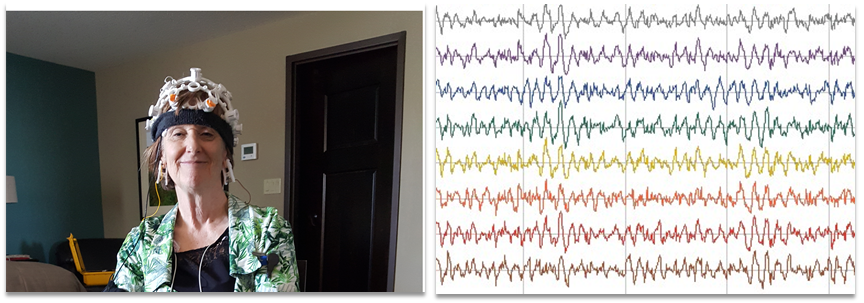 Image2: Open BCI based EEG collecting equipment mounted on a person during experiment and representational diagram of EEG signals
Let me start with a question? How many of you have seen your EEG signals? Only a few I guess and I really hope you never need to check your EEG at a hospital. I have seen mine, its quite an interesting signal. The picture you are seeing above is one of the EEG recording sessions conducted at our lab. We have setup our own EEG acquisition machine based on OpenBCI. The picture on right side demonstrate how an EEG signal looks like. EEG signals are included in the class of nonlinear dynamic signals. I’ll explain about that term later let’s see some neural diseases, Alzheimer’s, epilepsy and Parkinson’s are some neurodegenerative diseases that affect a lot of people. As the technology has advanced a lot of new ways to detect these diseases has discovered. Measuring EEG is a preferred method to diagnose many neural disorders. Recent studies has proposed that the brain state of a normal person is at the brink of chaos or more clearly in the mathematical sense brain state is more similar to the bifurcation of a complex chaotic system. And research works published on the above mentioned neural diseases proved that there is a notable change in the brain state. Our project goal is to build a wearable device, a small one like a pacemaker which can alter the brain signal patterns. It can be either invasive or non-invasive we haven’t gone that far to in our research yet. Chaotic systems are the closest type of nonlinear dynamic signals we can simulate for EEG signals. Hence our first step is to build a system that can model EEG signals, a simulator where we can test our functionalities. Hence as a trial study we design an Artificial Neural Network based system that can model any natural system given its inputs and outputs and use it to model Rossler’s and Chua’s chaotic system.
In this section we will see some of the recent literatures that have done similar studies:
1. Jesse Schmitz, Lei Zhang, Rossler based Chaotic communication system implemented on FPGA :30th Canadian Conference on Electrical and Computer Engineering (CCECE),IEEE. 2017
Conventional equation based modelling techniques are efficient but not suitable for empirical systems.
2. M. Alcin, I. Pehlivan, and smail Koyuncu, “Hardware design and implementation of a novel ann-based chaotic generator in fpga,” Optik - International Journal for Light and Electron Optics, vol. 127, no. 13, pp. 5500 – 5505, 2016.
For FPGA implementation of ANN 6 bit precision is sufficient
3. Archana R, A. Unnikrishnan R. Gopikakumari, M.V Rajesh, An Intelligent Computational Algorithm based on Neural Networks for the Identification of Chaotic systems :Recent Advances in Intelligent Computational Systems (RAICS),IEEE. 2011.
Larger number of hidden layer neurons are used. No performance evaluation of modelling ANN is done.
4. Lei Zhang, Artificial Neural Network Model Design and Topology Analysis for FPGA Implementation of Lorenz Chaotic Generator :30th Canadian Conference on Electrical and Computer Engineering(CCECE),IEEE. 2017.
Study done without considering consequences. Deep Neural Network used for modelling.
5. Razieh Falahian,Maryam Mehdizadeh Dastjerdi,et.al, Artificial neural network-based modeling of brain response to flicker light :Nonlinear Dyn,IEEE. 2015.
Bifurcation study not done. Open loop modelling technique.
- A comprehensive study on prediction and modelling of nonlinear dynamic systems using (1) Feedforward Neural Networks (2) Feedback Neural networks.
- How well the validation performance improves with increase in the number of hidden layer neurons?
- Which algorithm suites best for modelling complex nonlinear time series?
- Does the results hold for other dynamic systems?
- How well the modelled system performs in areas of timing and outputs?
Entire coding is done in MATLAB Neural Network Toolbox is used. MATLAb is wrapped version of Caffe.2 types of Neural Networks in FFNN (i) MLP (ii) RBFN and 2 types of feedback Neural Networks (i) TDNN (ii) RNN. Single hidden layer is deployed for all the Neural Networks. Training/Testing and Validation ratio used is 70:15:15. Loss function used is MSE and performance goals are calculated based on previous studies. Three dimensions of chaotic system are used for training & windowing method is used to generate training samples.
Feed forward Neural networks is the simple type of Artificial Neural Network where connections do not form a cycle as in Recurrent Neural Network. The flow of data is only in one direction, i.e. data is fed by the neurons from input layer to hidden layer then to output layer and there are no feedback connections between output and input. FFNN can be either single layer perceptron model (SLP) or Multilayered perceptron (MLP). RBFN is another member of the feedforward neural network and has Radial basis function as activation function. Radbas function are used for function approximation, classification and prediction. It has both unsupervised and supervised phases.
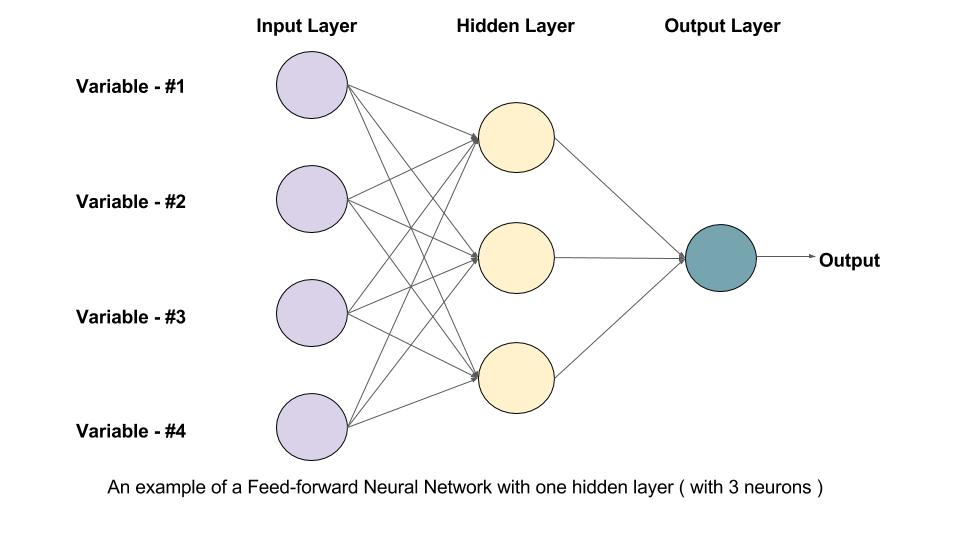
Image3: AN example of a feedforward Neural Network with a hidden layer of 3 neurons
First 10k training samples are ignored in order to remove any transient noise. Hyperbolic tangent sigmoid and linear linear activation are used for hidden and output layer of MLP respectively. Gaussian activation function is used in the funtional layer of Radial Basis Function Network. Each experiment run for 1000 epochs and multiple trials to avoid gradient hitting local minima with 6 validation stops. RBFN MSE is calculated for different values of spread & value with minimum MSE chosen.
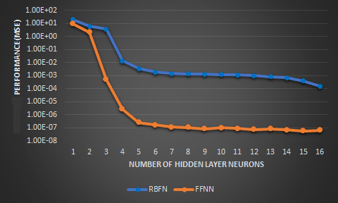
Image4: Validation performance comparison plot of RBFN vs FFNN for the Rossler’s system
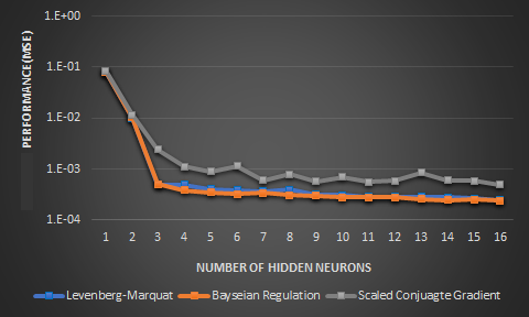
Image5: Validation performance of FFNN over different learning algorithms for the Chua’s map
For all architectures the testing performance improves as the hidden layer neurons increase. MSE comparison between MLP and RBFN is done at 2.00E-06. MLP took 5 neurons while RBFN took 20 neurons to reach same performance. Out of the three algorithm tested LM algorithm is found as the best algorithm: (i) rate of convergence (ii) training time. Testing performance doesn't improve a lot after 8 hidden neurons. Chua’s system results followed Rossler’s. FFNN MSE3E-04.
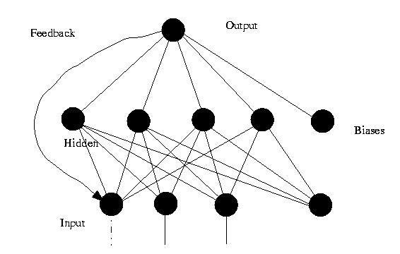
Image6: AN example of a feedback Neural Network with a hidden layer of 4 neurons
NAR neural network can be trained to forecast the next values from the information of that series past value. Training of the network is done in open loop form and prediction is done in closed loop form. NAR network is trained in open loop on the data of the Rossler’s chaotic system. The input time delay is experimentally determined as one. The architecture has only one input and in closed loop mode input is joined to the output. We execute the closed loop architecture by giving just the input delay and initial values. This is identical to a chaotic system iteration where we only need the initial values to iterate through the trajectories. The performance of the closed loop model over different trials for LM algorithm is given in the plot below. LM algorithm is chosen here because its performance was found optimal for open loop training which is the first part of the NAR training also. Trial and error method is employed to calculate the best input delay and as delay increases, there are 2 drawbacks. There is an increase in the training time for the neural network as convergence rate also decreases and the performance also degrades since the prediction can be either depend on short term or long-term memory of the input time series. Hence single delay is selected as most effective one for our scenario. NARX are dynamic recurrent neural networks that can successfully use its output feedback loop to improve its predictive performance in complex time series prediction and modelling tasks. It has been proved in previous studies that NARX network outperform NAR networks in prediction accuracy due to its external input which serves as a real data input and enhance further prediction accuracy. In this study a repetition of this is not done, instead a novel modelling technique for the bifurcation diagram of Rossler’s system is studied. Bifurcation diagrams explain the illustrates the summary of succession of period doubling process with the change in the parameter.
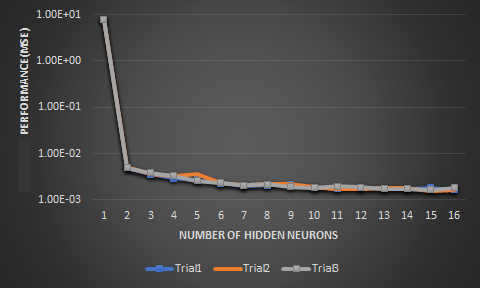
Image7: Validation performance of NAR ANN over different trials for Rossler’s chaotic map
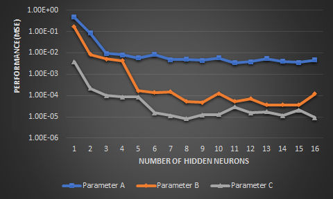
Image8: Validation performance comparison of Rossler’s bifurcation for parameters a,b,c vs number of neurons for NARX ANN
Time delayed Neural Network The Nonlinear Auto-Regressive(NAR) for generating an iterative model. Dynamic Recurrent Neural Network Nonlinear Auto-Regressive with Exogenous Inputs (NARX). Single input to the NARX is the bifurcation parameter of Rossler’s map. Input delay and target delay are experimentally calculated as 1 time step.
The chaotic model performance need to be evaluated to ensure the output of the neural network model is correct and the neural network is sufficiently trained. Loss function ensures the performance of the neural network, but a quantitative study and qualitative study will help to visualize and compare the outputs of neural network model and empirical system. Quantitative analysis of the data includes measuring the volatility of the system, which includes the degree of variations in the data. This can be measured by analyzing the Hurst exponent and Lyapunov exponent of the empirical data. Hurst exponent analysis is mainly used for identifying trends, deterministic chaos and fractal structure of data. Lyapunov exponents measure the rate of separation of very close trajectories, which means they can be very helpful in understanding the degree of sensitivity to initial conditions. On the other hand, qualitative analysis of the system includes superposition of the output of the neural network model over the empirical data. This provides a visual representation of the accuracy of state space model of the modelled chaotic system. Finally, the effectiveness of the neural network model is evaluated by a runtime analysis to measure the time it takes to generate the state space model once trained.
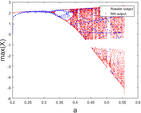
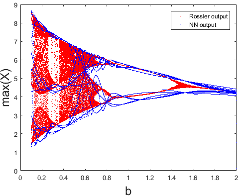
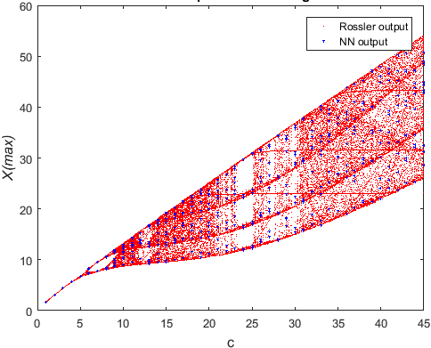
Image9: Output time series and bifurcation diagrams w.r.t parameter a, b, c are reconstructed using the dynamic NN model
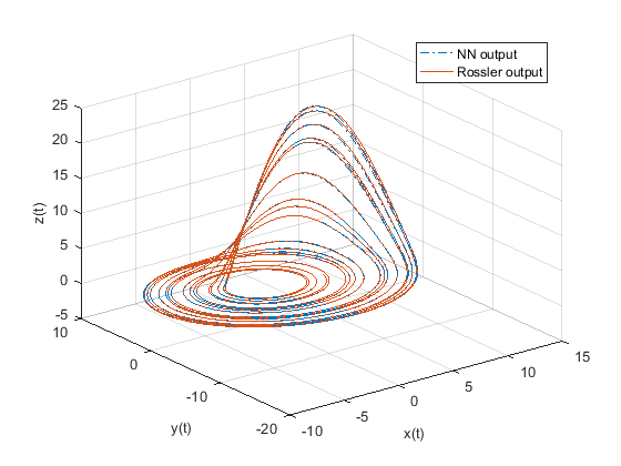
Image10: State diagram of NN model superimposed on actual Rossler’s attractor
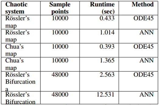
Table1: Runtime comparison between ODE method and NN generated chaotic models