===================== Vectorization of ArcInfo Grid ASCII files as ESRI Shapefiles. Python program to convert an ArcInfo Grid ASCII raster file to an ESRI shapefile in one of two formats:
- with a single layer containing oriented grid square polygons centered at the pixels of the grid; and
- with a single layer containing "dissolved" polygons. The dissolve is performed in the (row, column) coordinates of the raster space.
Each polygon contains an attribute value equal to the value of the corresponding pixel of the ArcInfo Grid ASCII raster file.
The ArcInfo Grid ASCII header cellsize parameter
determines the size of the grid squares.
In contrast to the ArcGIS Raster to Polygon and the gdal_polygonize.py
raster to polygon feature layer conversion utilities, aig2shp.py does not require
float raster values to be discretized into (nonnegative) integer values before conversion. Your
raster data is preserved, which may have some advantages for geospatial analysis. Nevertheless,
the vector files are large, so arcinfo.py is available to reclassify ArcInfo Grid ASCII raster
files.
The program was written to upload raster data in a format useable by CartoDB. See the following correspondence on the CartoDB google group.
The following was determined from ESRI documentation of ArcInfo Grid ASCII
files online, and was verified by examination of the output of the
gdalinfo GDAL utility applied to ArcInfo Grid ASCII files, and
by examination of converted files within GIS systems.
- The origin of the raster is defined to be the
(x, y)coordinates of the upper-left corner of the upper left grid square of sizecellsize, namely(x0, y0) = (xllcorner, yllcorner + nrows * cellsize). - The coordinates of the center of the grid square at the origin are then
(x0 + cellsize/2, y0 - cellsize/2). - In general, the geographic coordinates
(x, y)of the pixel at(row, col)are given by(x, y) = (xllcorner + (col + 1/2) * cellsize, yllcorner + (nrows - row - 1/2) * cellsize).
The dissolve operation embeds the pixel matrix into a box space with additional coordinates for the vertices of the grid squares centered at each pixel. The coordinates of a point in box space are denoted [r,c]. The change of coordinates is given by
[r, c] = [2i+1, 2j+1],
where (i, j) are the coordinates of the pixel at row i, column j in raster space. The four corners and edge coordinates of the box corresponding to the pixel (i, j) are shown below. The directions shown are clockwise traversal directions at each vertex.
 UL→   Top   UR↓       [r-1,c-1]  [r-1,c] [r-1,c+1]
 Left  [r,c] Right     [r,c-1]    [r,c]   [r,c+1]
 LL↑   Bot   LR←       [r+1,c-1]  [r+1,c] [r+1,c+1]
The edges, denoted Top, Right, Bot and Left, aren't used (4/9ths wasted). The geographic coordinates of the vertex at [r,c] are given by
(x, y) = (xllcorner + cellsize * (c / 2 ), yllcorner + cellsize * (nrows - (r / 2))
An advantage of computation in box space is that vertices have even coordinates, so division by 2 can be done by right shifting. The conversion to geographic coordinates is postponed until the shapefile is written.
usage: aig2shp.py [-h] [-a attribute] [-d] [-e minX minY maxX maxY] [-l LAYER]
                  [-n] [-O] [-q] [-v] [--version] [--wgs84]
                  grid_ASCII_file ESRI_shapefile

Create ESRI Shapefile from ArcInfo Grid ASCII raster.

positional arguments:
  grid_ASCII_file       ArcInfo Grid ASCII input file.
  ESRI_shapefile        ESRI shapefile output file.

optional arguments:
  -h, --help            show this help message and exit
  -a attribute, --attr attribute
                        Name of attribute for ArcInfo grid values. Defaults to
                        "value."
  -d, --dissolve        Dissolve ArcInfo ASCII Grid in raster space before
                        converting to shapefile. Saves space, usually.
  -e minX minY maxX maxY, --extent minX minY maxX maxY
                        Bounding box of subset of raster in geographic
                        coordinates.
  -l LAYER, --layer LAYER
                        Shapefile layer name string. Default is grid_value.
  -n, --nonzero         Exclude zero values.
  -O, --opt             Enable greedy cell marking optimization.
  -q, --quiet           Suppress progress bar.
  -v, --verbosity       Display verbose message output. Each additional 'v'
                        increases message verbosity: -vv is very verbose, and
                        -vvv is very very verbose.
  --version             Show program version number and exit.
  --wgs84               Set spatial reference to WGS84/EPSG:4326 in shapefile
                        layer. Projection file (.prj) is written out.

Software is released under The MIT License (c) 2013 Florian Lengyel, CUNY
Environmental CrossRoads Initiative, Advanced Science Research Center, The
City College of New York. Contact: gmail/skype/twitter florianlengyel.
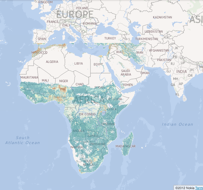
In this example, cropland for a region including Africa was subsetted from the Ramankutty cropland raster data set [1] in ArcInfo Grid ASCII format, and used to produce a corresponding shapefile.
./aig2shp.py -e -17.338675 -34.892837 57.845763 37.428152 \
--wgs84 -n -v ramankutty_cropland2000_frac_5m.asc vector_squares.shp
The shapefile was uploaded to CartoDB; a screenshot is shown below.

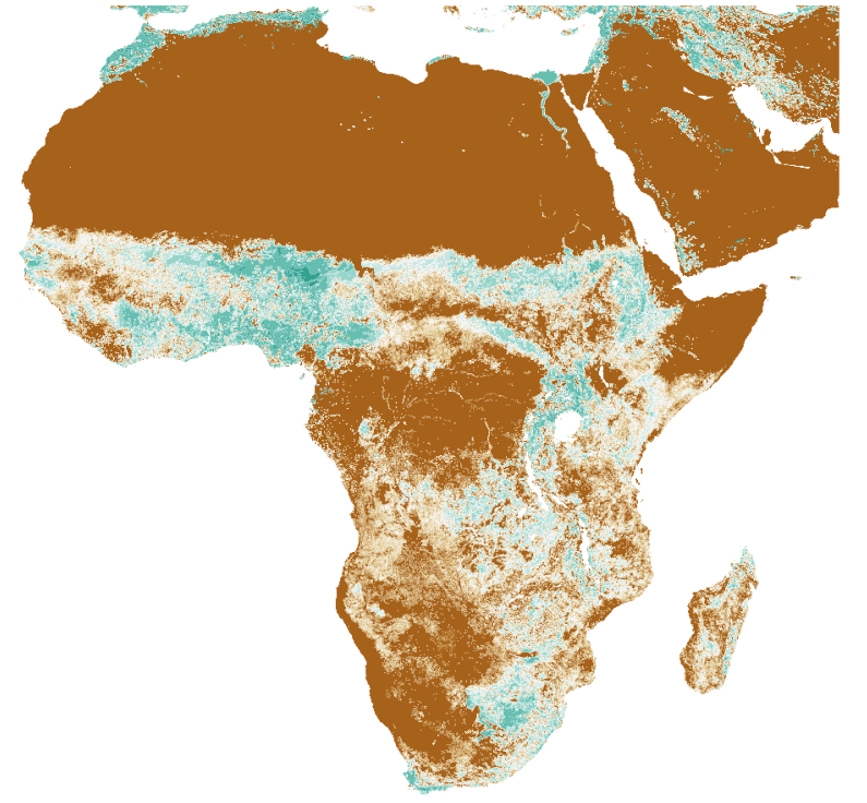
The previous example results in large files, with one vector grid square per raster pixel. Polyonalization produces a better result, after quantile reclassification.
./arcinfo.py -s 1000 -b 20 -r qu \
	-e -17.338675 -34.892837  57.845763  37.428152 \
	ramankutty_cropland2000_frac_5m.asc croplandeq20.asc

./aig2shp.py -d -vv --wgs84 croplandeq20.asc test.shp
ogrinfo shows 3643 polygons, as opposed to 88917 for the previous example.
INFO: Open of `test.shp'
      using driver `ESRI Shapefile' successful.

Layer name: test
Geometry: 3D Polygon
Feature Count: 3643
Extent: (-11.600000, 4.200000) - (15.800548, 23.900394)
Layer SRS WKT:
GEOGCS["GCS_WGS_1984",
    DATUM["WGS_1984",
        SPHEROID["WGS_84",6378137,298.257223563]],
    PRIMEM["Greenwich",0],
    UNIT["Degree",0.017453292519943295]]
- ProgressBar
- GDAL 1.9.1 GDAL Python bindings
- numpy 1.0.0 or greater
- scipy (for arcinfo.py)
- argparse
There are several opportunities for functional and object-oriented improvements.
-
Box coordinates can be handled through an interface. The box coordinate
[r,c]is valid if and only ifr+cis even. The point[r,c]is the box coordinate of a vertex if and only ifrandcare even. The point[r,c]is the box coordinate of a region number (corresponding to a pixel in raster space) if and only ifrandcare odd. -
The interface to the box space could be a class. The implementation need not be a directly manipulated matrix of size
(2nrows+1)x(2ncols+1). The vertex space need not be implemented as an array, but as a single point whose coordinates vary from vertex to vertex as the point moves through the box coordinate space. At most two points are needed: the next valid point, and the currently moving point. Only centroids of boxes are ever written to. Vertices in box space never have values, so values of vertices need not be represented at all. -
Region numbers are the (centroid) values of boxes. Region numbers could be stored in a matrix of size
nrows x ncols. The mapping from internal coordinates to external box centroid coordinates is[r,c] = {2p+1,2q+1}. The change of coordinates between raster space(i,j)coordinates and internal box centroid coordinates is the identity. -
DONE: The internal box centroid space could be represented by a matrix of 32-bit integers. This is necessary because there can be hundreds of thousands or millions of polygons in general, and there is a one-one correspondence between regions and polygon boundaries (but not holes). Sixteen-bit words are insufficient. However, the use of one 32-bit arrays for box centroid values will save considerable space. Conceptually, such an interface presents this pattern of coordinates:
 UL→     UR↓     [r-1,c-1]     [r-1,c+1]
.  [r,c]                 [r,c]
 LL↑     LR←     [r+1,c-1]     [r+1,c+1]
Nothing more is needed. The box coordinate [r,c] automatically satisfies r+c = 0 mod 2. The internal representation is never manipulated directly--always through a stylized interface.
-
The traversal algorithm depends on a box coordinate [r, c] that moves from vertex to vertex. This pair of coordinates could be an object which moves according to a direction v. We might as well write
x.move(v). A test for equality is needed. -
The traversal algorithm itself should be abstracted, with provisions for functional actions at each turn (when the initial and final directions change) and for a preamble.
-
Region number handling could be abstracted and possibly handled together with the polygon database, which maps a region number to the starting vertex of the boundary of the polygon having that region number. The region to class mapping can also be handled. A region number can be provisionally assigned through such an interface, and then commited if there are no path collisions, or reverted if there is a path collision.
Florian Lengyel, CUNY Environmental CrossRoads Initiative, Advanced Science Research Center, The City College of New York, CUNY. Contact: gmail/skype/twitter florianlengyel
Dorsey Davidoff's suggestions were incorporated in the algorithms.
Tian Luan suggested a revision to eliminate an extra colinear point in the construction of holes of polygons.
Original software is licensed under the MIT License: (c) 2013 Florian Lengyel and Dorsey Davidoff. All other original work is licensed under an Attribution-NonCommercial-ShareAlike 3.0 United States Creative Commons License: (CC BY-NC-SA 3.0 US) 2013 Florian Lengyel. Derivative work is licensed accordingly. Full license in License.txt.
