About

In this repository you can find algorithms & data structures in the pure JavaScript language.

The goal is to systematize and consolidate knowledge of algorithms.

Table of contents:

Well-known algorithms

1. Sorting algorithms

1.1 Bubble sort

1.2 Quicksort

1.3 Mergesort

1.4 Selection sort

1.5 Heapsort

1.6 Shellsort

1.7 Insertion sort

2. Search algorithms
3. Graph algorithms
4. Permutation algorithms
5. Various algorithms

Computational complexity

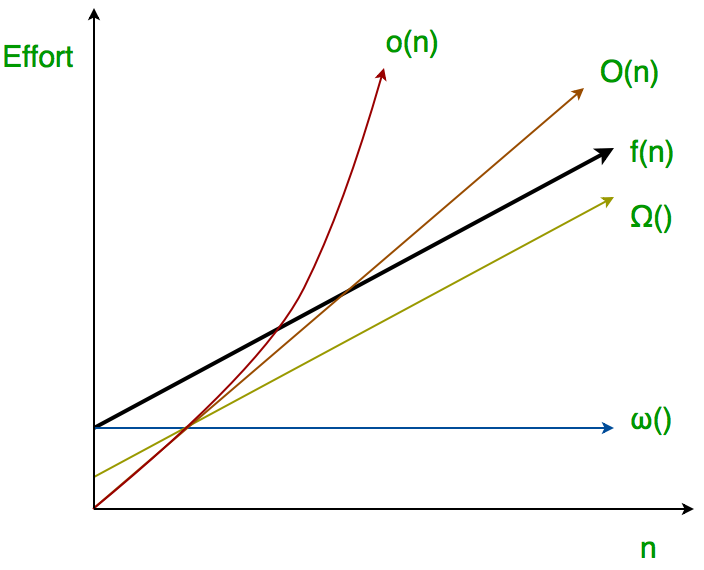
1. Description of the kinds of bounds on asymptotic growth rates
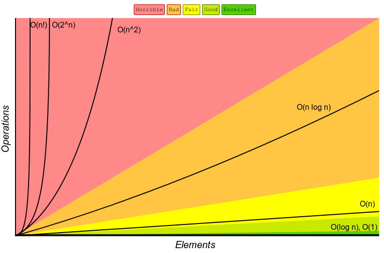
2. Common orders of growth
3. Computational complexity of algorithms

Leetcode

1. Pascal's triangle
2. Single number
3. Happy number
4. Valid Palindrome
5. Valid Anagram
6. Path Sum
7. Add One Row to Tree
8. Largest Perimeter Triangle
9. Delete Node in a Linked List
10. Check if the Sentence Is Pangram
11. Integer to Roman
12. Contains Duplicate II

Codewars

Well-known algorithms

Sorting algorithms:

1. Bubble sort

   

   #adaptive sort

   #comparison-based

• Simple bubble sort
• Optimized bubble sort

2. Quicksort

   

   #in-place

   #unstable sorting

   #divide and conquer

   #comparison-based

• Quick sort with built-in methods
• Pure quick sort
• Classic quick sort (Hoare partition scheme)
• Optimized classic quick sort (Hoare partition scheme)

3. Merge sort

   

   #divide and conquer

   #stable sorting

   #comparison-based

• Merge sort

4. Selection sort

   

   #comparison-based

• Selection sort with list structure and built-in methods
• Pure selection sort

5. Heapsort

   

   #comparison-based

6. Shellsort

   

   #comparison-based

7. Insertion sort

   

   #comparison-based

• Insertion sort

Search algorithms:

1. Binary search

• Iterative binary search
• Recursive binary search

2. Largest & smallest element in an array

• Find largest element in an array
• Find smallest element in an array

3. Second largest & smallest element in an array

• Find second largest element in an array
• Find second smallest element in an array

Graph algorithms:

1. Breadth First Search (BFS)
2. Depth First Search (DFS)
3. Dijkstra
4. Bellman Ford's algorithm

Permutation algorithms:

1. Fisher–Yates shuffle (Knuth)
2. Reverse

Various algorithms

1. Fizz Buzz

Computational complexity

Computational complexity is a complexity that expresses the dependence of the algorithm's workload on the input data. The amount of work includes time and space (the amount of memory) computational complexity. This area attempts to answer the central question of algorithm design: "how will the execution time and the amount of memory occupied change depending on the size of the input?" The main classes of complexity are:

Class P - problems for which there are fast solutions - sorting, array searching, matrix multiplication, and others. Algorithms of class P are called polynomial - the running time of which does not depend too much on the size of the input data (that is, the time does not exceed the polynomial of the data size).

Class NP - In the theory of algorithms class NP (from non-deterministic polynomial) is a set of decidability problems (where you can answer is solvable or not), whose solution can be checked on the Turing machine in time, not exceeding the value of a polynomial of the size of the input data, in the presence of some additional information (the so-called solution certificate). Any problem of class NP can be solved by brute force (kind of like bruteforcing, exponential complexity). Roughly speaking, these are complex problems that take a very long time to solve(factorial, exponential) and for which there is no optimally fast algorithm. Examples: Hamiltonian path problem, the traveling salesman problem.

Time complexity - computation complexity, that is defined from the input data determining the number of operations and equal to the algorithm's running time with the given input data. The time complexity of an algorithm is usually expressed using asymptotic analysis.
Not to be confused with runtime which describes how much time it takes to execute a program on a specific computing machine, while the time complexity is not tied to the actual execution time and the current computer on which the algorithm will be executed.

Space complexity - computation complexity, that describe amount of memory space required to solve an instance of the computational problem as a function of characteristics of the input. In other words, it is the memory required by an algorithm until it executes completely. Similar to time complexity, space complexity is often expressed asymptotically in big O notation.

Asymptotic analysis is a complexity analysis for input data that tends to infinity. It is expressed in notations (O(big O), Ω(omega), Θ(theta)). In most cases, big O notation is used, which defines the worst case (upper limit from function growth) and does not take into account constants.

---

Description of the kinds of bounds on asymptotic growth rates

Let f and g be functions from positive integers to positive integers. Then:

Designation	Bound	Efficiency compared to the real complexity of the algorithm
Θ; f(n) = Θ(g(n)), if there exists a positive integer n0 and a positive constants c1 > 0 and c2 > 0, such that c1 * g(n) ≤ f(n) ≤ c2 * g(n) ∀ n>n0	Lower and upper bounds, accurate estimate	Equal
О; f(n) = О(g(n)), if there exists a positive integer n0 and a positive constant c > 0, such that f(n)≤cg(n) ∀ n≥n0	Upper bound, but this bound might or might not be a supremum	Less or equal
o; f(n) = o(g(n)), if there exists a positive constant c > 0, such that f(n)≤cg(n) ∀ but perhaps finitely many n	Upper bound, not an accurate estimate	Less
Ω; f(n) = Ω(g(n)), if there exists a positive integer n0 and a positive constant c > 0, such that cg(n)≤f(n) ∀ n>n0	Lower bound, but this bound might or might not be a infimum	Greater or equal
ω, f(n) = ω(g(n)), if there exists a positive constant c > 0, such that cg(n)≤f(n) ∀ but perhaps finitely many n	Lower bound, not an accurate estimate	Greater

"Ο(f(n))" implies that as the amount of input data n increases, the running time of the algorithm will increase no faster than some constant multiplied by f(n).

Common orders of growth

The order of growth of an algorithm is a rough estimate of the time/memory required to execute a computer program as the size of the input data changes.
Growth order ignores the constant factor needed for fixed operations and focuses on operations that increase in proportion to the size of the input data.

Function	Type of Growth	Example
1	constant	Finding the median value in a sorted array of number
n	linear	Finding the smallest or largest item in an unsorted array
log n	logarithmic	Binary search
n log n	linearithmic	Fast Fourier transform
n^2	quadratic	Bubble sort
n^3	cubic	Naive multiplication of two n * n matrices
2^poly(n)	exponential	Solving matrix chain multiplication via brute-force search
n!	factorial	Solving the traveling salesman problem via brute-force search

Reference - Big-O Cheat Sheet

---

Computational complexity of algorithms

Sorting algorithms

Algorithm	Time complexity			Space complexity
*	Best	Average	Worst	Worst
Quicksort	Ω(n log(n))	Θ(n log(n))	O(n^2)	O(n), optimized O(log(n))
Mergesort	Ω(n log(n))	Θ(n log(n))	O(n log(n))	O(n)
Timsort	Ω(n)	Θ(n log(n))	O(n log(n))	O(n)
Heapsort	Ω(n log(n))	Θ(n log(n))	O(n log(n))	O(1)
Bubble Sort	Ω(n)	Θ(n^2)	O(n^2)	O(1)
Insertion Sort	Ω(n)	Θ(n^2)	O(n^2)	O(1)
Selection Sort	Ω(n^2)	Θ(n^2)	O(n^2)	O(1)
Tree Sort	Ω(n log(n))	Θ(n log(n))	O(n^2)	O(n)
Shell Sort	Ω(n log(n))	depends on gap sequence, in general: Θ(n(log(n))^2)	depends on gap sequence: O(n(log(n))^2) or O(n^2)	O(1)
Bucket Sort	Ω(n+k)	Θ(n+k)	O(n^2)	O(n)
Radix Sort	Ω(nk)	Θ(nk)	O(nk)	O(n+k)
Counting Sort	Ω(n+k)	Θ(n+k)	O(n+k)	O(k)
Counting Sort	Ω(n)	Θ(n log(n))	O(n log(n))	O(n)

---

Leetcode:

Problem: Pascal's triangle

Solution: https://github.com/pavlokolodka/algorithms/blob/8aeec8dcc2c65927d32430990de27b0de4dc3eb3/leetcode/pascalstriangle.js

Problem: Single number

Solution: https://github.com/pavlokolodka/algorithms/blob/526164437a75610e4f0453dfcfb2b121373001ec/leetcode/singlenumber.js

Problem: Happy number

Solution: https://github.com/pavlokolodka/algorithms/blob/6afd702aa179f03d670671790426ac8a8021361d/leetcode/happynumber.js

Problem: Valid Palindrome

Solution: https://github.com/pavlokolodka/algorithms/blob/915f34a7eafede3a97b0ba35b297aa03beca58f0/leetcode/validpalindrome.js

Problem: Valid Anagram

Solution: https://github.com/pavlokolodka/algorithms/blob/48a5862b096ee35c7cdecd039059da7b71560444/leetcode/validanagram.js

Problem: Path Sum

Solution: https://github.com/pavlokolodka/algorithms/blob/d5e1f84ab03f371261621b8cae72714a4fc63d3f/leetcode/pathsum.js

Problem: Add One Row to Tree

Solution: https://github.com/pavlokolodka/algorithms/blob/fcc2a140880de6a6dd32ae5183c1c6dc6b0a76a1/leetcode/addOneRowToTree.js

Problem: Largest Perimeter Triangle

Solution: https://github.com/pavlokolodka/algorithms/blob/01f9a31b8a5a1d517caf791a2ace6a807d996133/leetcode/largestPerimeterTriangle.js

Problem: Delete Node in a Linked List

Solution: https://github.com/pavlokolodka/algorithms/blob/8104920f3dcfb7ccbeda935678cf66869d65d31c/leetcode/deleteNodeInLinkedList.js

Problem: Check if the Sentence Is Pangram

Solution: https://github.com/pavlokolodka/algorithms/blob/13481038f34f7ee1f3e67f15e924dce65b20e55d/leetcode/%D1%81heckIfTheSentenceIsPangram.js

Problem: Integer to Roman

Solution: https://github.com/pavlokolodka/algorithms/blob/824cd492a95f58b924a6e0a2211ba2f4267b6750/leetcode/integerToRoman.js

Problem: Contains Duplicate II

Solution: https://github.com/pavlokolodka/algorithms/blob/0dc7fff9ce3ff49b906df19e9c3d01f52e7abcc9/leetcode/containDuplicateII.js