Example
The experiments folder contains some scripts for a comparison of online learning algorithms, as well as the comparison with another two toolboxes: VW and LIBLINEAR. We provided examples on four datasets, from small scale low dimensional to large scale high dimensional. The dataset sizes are:
| dataset | #train | dim | #class |
|---|---|---|---|
| a1a | 1605 | 119 | 2 |
| mnist | 60000 | 780 | 10 |
| rcv1 | 677399 | 47236 | 2 |
| url | 2146552 | 3231961 | 2 |
| webspam | 300000 | 16609143 | 2 |
The training time of SOL(OGD and AROW algorithm), VW and LIBLINEAR are:
| dataset | SOL(OGD) | SOL(AROW) | VW | LIBLINEAR |
|---|---|---|---|---|
| a1a | 0.0019 | 0.0018 | 0.0571 | 0.0356 |
| mnist | 1.4724 | 1.4680 | 1.8747 | 145.5023 |
| rcv1 | 8.4109 | 8.4390 | 11.3581 | 77.9274 |
| url | 12.1774 | 13.6496 | 24.8073 | 893.8768 |
| webspam | 203.5114 | 198.9504 | 249.3320 | 1708.8001 |
The test accuracy of SOL(OGD algorithm), VW and LIBLINEAR are:
| dataset | SOL(OGD) | SOL(AROW) | VW | LIBLINEAR |
|---|---|---|---|---|
| a1a | 0.8363 | 0.8402 | 0.8326 | 0.8425 |
| mnist | 0.9171 | 0.9226 | 0.9125 | 0.9183 |
| rcv1 | 0.9727 | 0.9766 | 0.9754 | 0.9771 |
| url | 0.9844 | 0.9940 | 0.9897 | 0.9960 |
| webspam | 0.9888 | 0.9955 | 0.9944 | 0.9931 |
To quikly get a comparison on the small dataset "a1a" as provided in the data folder:
$ cd experiments
$ python experiment.py --shufle 10 a1a ../data/a1a ../data/a1a.t
The script will conduct cross validation to select best parameters for each algorithm. Then the script will shuffle the training 10 times. For each shuffled data, the script will train and test for each algorithm. The final output is the average of all results. And a final table report will be shown as follows.
algorithm   train           train           test            test
            accuracy        time(s)         accuracy        time(s)
pa1         0.8011+/-0.0058 0.0029+/-0.0029 0.8193+/-0.0103 0.0152+/-0.0013
pa2         0.7913+/-0.0062 0.0018+/-0.0001 0.8013+/-0.0200 0.0146+/-0.0011
eccw        0.7950+/-0.0067 0.0018+/-0.0001 0.7985+/-0.0097 0.0155+/-0.0016
arow        0.8211+/-0.0061 0.0018+/-0.0001 0.8402+/-0.0009 0.0147+/-0.0009
pa          0.7759+/-0.0097 0.0018+/-0.0001 0.7758+/-0.0329 0.0151+/-0.0011
sop         0.7816+/-0.0073 0.0019+/-0.0001 0.7840+/-0.0189 0.0152+/-0.0007
ada-fobos   0.8055+/-0.0052 0.0019+/-0.0001 0.8234+/-0.0043 0.0149+/-0.0009
ada-rda     0.8114+/-0.0032 0.0019+/-0.0001 0.8347+/-0.0049 0.0147+/-0.0008
rda         0.7528+/-0.0008 0.0019+/-0.0002 0.7595+/-0.0000 0.0145+/-0.0009
erda        0.8049+/-0.0055 0.0019+/-0.0001 0.8326+/-0.0067 0.0146+/-0.0013
cw          0.7913+/-0.0065 0.0018+/-0.0001 0.7907+/-0.0113 0.0149+/-0.0010
vw          0.8443+/-0.0082 0.0571+/-0.0683 0.8326+/-0.0069 0.2582+/-0.0310
alma2       0.8087+/-0.0037 0.0017+/-0.0001 0.8263+/-0.0089 0.0153+/-0.0013
ogd         0.8108+/-0.0041 0.0019+/-0.0001 0.8363+/-0.0020 0.0150+/-0.0010
perceptron  0.7713+/-0.0054 0.0017+/-0.0001 0.7793+/-0.0187 0.0151+/-0.0009
liblinear   0.8536+/-0.0000 0.0356+/-0.0028 0.8425+/-0.0000 0.5620+/-0.0036
The number of updates with respect to the training iterations are: 
The training error rate with respect to the training iterations are: 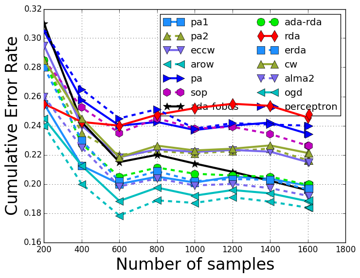
To compare the sparse online learning algorithms, the test error rate compared to the model sparsity is: 
Users can also compare on the multi-class dataset "mnist" with the follow command (Note that we only shuffle the training data once in this example, so the standard deviation is zero):
$ python experiment.py mnist ../data/mnist.scale ../data/mnist.scale.t
The output is:
algorithm   train           train           test            test
            accuracy        time(s)         accuracy        time(s)
pa1         0.8553+/-0.0009 1.4840+/-0.0163 0.8753+/-0.0164 0.2474+/-0.0018
pa2         0.8585+/-0.0008 1.4804+/-0.0228 0.8811+/-0.0131 0.2469+/-0.0040
eccw        0.8764+/-0.0210 1.4825+/-0.0167 0.8688+/-0.0493 0.2468+/-0.0030
arow        0.9051+/-0.0004 1.4680+/-0.0136 0.9226+/-0.0014 0.2458+/-0.0038
perceptron  0.8460+/-0.0008 1.4752+/-0.0151 0.8671+/-0.0164 0.2483+/-0.0052
ada-rda     0.8999+/-0.0005 1.4736+/-0.0090 0.9201+/-0.0022 0.2467+/-0.0047
ada-fobos   0.9055+/-0.0007 1.4807+/-0.0196 0.9239+/-0.0020 0.2468+/-0.0027
pa          0.8553+/-0.0009 1.4667+/-0.0210 0.8753+/-0.0164 0.2465+/-0.0023
sop         0.8552+/-0.0007 1.4751+/-0.0149 0.8811+/-0.0099 0.2481+/-0.0054
rda         0.7868+/-0.0009 1.4630+/-0.0166 0.8027+/-0.0027 0.2483+/-0.0018
cw          0.8784+/-0.0008 1.4784+/-0.0240 0.8861+/-0.0034 0.2459+/-0.0044
vw          0.9138+/-0.0023 1.8747+/-0.0743 0.9125+/-0.0019 0.3252+/-0.0121
ogd         0.8943+/-0.0009 1.4724+/-0.0192 0.9171+/-0.0008 0.2481+/-0.0039
alma2       0.8972+/-0.0008 1.4723+/-0.0134 0.9188+/-0.0022 0.2498+/-0.0118
erda        0.8839+/-0.0005 1.4707+/-0.0120 0.9132+/-0.0042 0.2474+/-0.0017
liblinear   0.9263+/-0.0001 145.5023+/-17.7614 0.9183+/-0.0001 2.0172+/-0.0164
The number of updates with respect to the training iterations are: 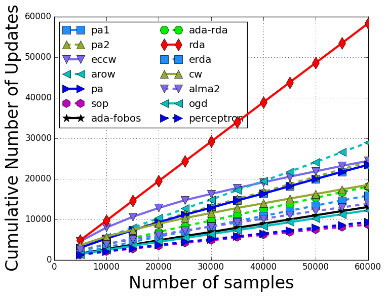
The training error rate with respect to the training iterations are: 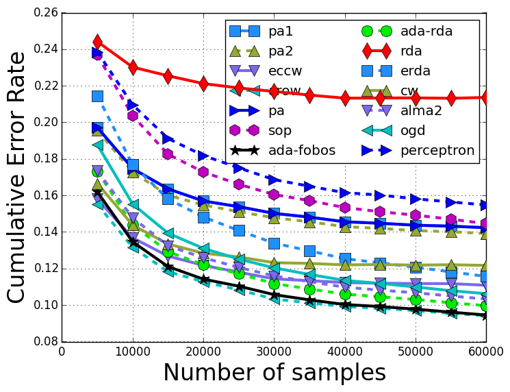
To compare the sparse online learning algorithms, the test error rate compared to the model sparsity is: 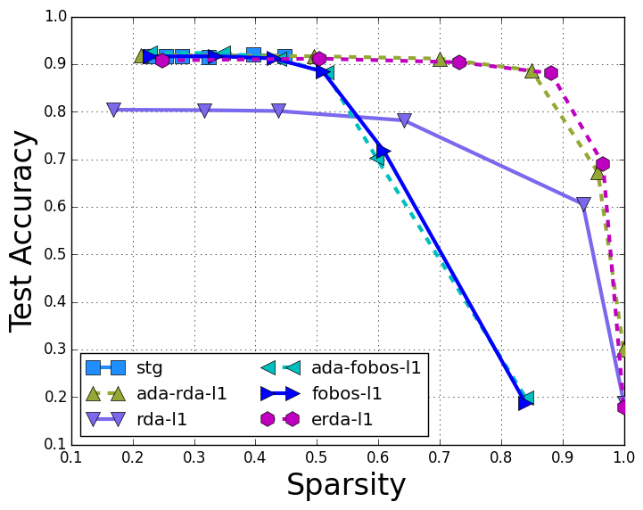
The tables and figures in our paper description are obtained on the "rcv1" dataset with the following command (we change the role of rcv1_train and rcv1_test, since rcv1_test has many more samples):
$ python experiment.py --shuffle 10 rcv1 ../data/rcv1_train ../data/rcv1_test
The output is:
algorithm   train           train           test            test
            accuracy        time(s)         accuracy        time(s)
pa1         0.9739+/-0.0001 8.5113+/-0.1143 0.9760+/-0.0005 0.2753+/-0.0051
pa2         0.9732+/-0.0001 8.4445+/-0.1068 0.9758+/-0.0003 0.2735+/-0.0034
eccw        0.9702+/-0.0001 8.4641+/-0.1116 0.9681+/-0.0009 0.2714+/-0.0062
arow        0.9754+/-0.0001 8.4390+/-0.1292 0.9766+/-0.0002 0.2737+/-0.0041
pa          0.9661+/-0.0002 8.4506+/-0.1031 0.9649+/-0.0015 0.2746+/-0.0045
sop         0.9610+/-0.0001 8.5246+/-0.1017 0.9627+/-0.0012 0.2757+/-0.0041
ada-fobos   0.9751+/-0.0001 8.4897+/-0.0872 0.9769+/-0.0003 0.2739+/-0.0040
ada-rda     0.9750+/-0.0001 8.4388+/-0.1140 0.9767+/-0.0003 0.2718+/-0.0070
rda         0.9229+/-0.0003 8.4809+/-0.0899 0.9212+/-0.0000 0.2729+/-0.0044
erda        0.9445+/-0.0001 8.4623+/-0.1123 0.9493+/-0.0002 0.2714+/-0.0057
cw          0.9678+/-0.0002 8.4356+/-0.1118 0.9656+/-0.0010 0.2697+/-0.0067
vw          0.9837+/-0.0002 11.3581+/-0.3423 0.9754+/-0.0009 0.4395+/-0.0193
alma2       0.9722+/-0.0001 9.1464+/-0.1624 0.9745+/-0.0005 0.2739+/-0.0043
ogd         0.9691+/-0.0005 8.4109+/-0.0982 0.9727+/-0.0006 0.2709+/-0.0055
perceptron  0.9607+/-0.0001 8.4296+/-0.0867 0.9625+/-0.0014 0.2742+/-0.0041
liblinear   0.9839+/-0.0000 77.9274+/-1.4742 0.9771+/-0.0000 2.1305+/-0.0305
The number of updates with respect to the training iterations are: 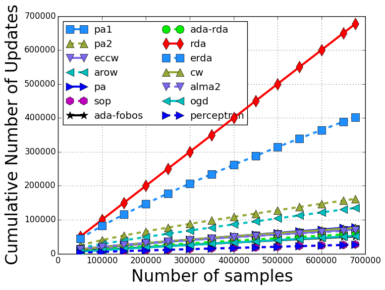
The training error rate with respect to the training iterations are: 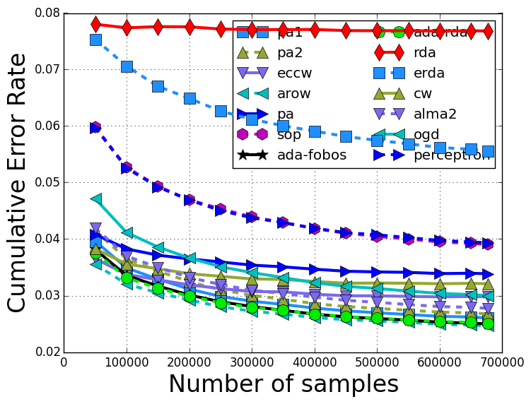
To compare the sparse online learning algorithms, the test error rate compared to the model sparsity is: 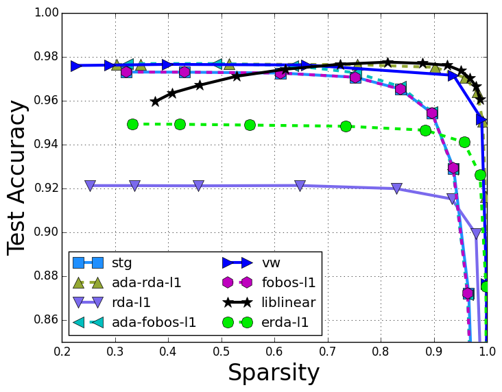
We also experiment on a much larger dataset "url". Here we only show the training time and test accuracies. Similar observations can be observed as above figures.
$ python experiment.py --shuffle 1 rcv1 ../data/rcv1_train ../data/rcv1_test

algorithm   train           train           test            test
            accuracy        time(s)         accuracy        time(s)
pa1         0.9778+/-0.0000 12.1930+/-0.0000 0.9827+/-0.0000 1.2261+/-0.0000
pa2         0.9783+/-0.0000 12.4444+/-0.0000 0.9834+/-0.0000 1.2342+/-0.0000
eccw        0.9852+/-0.0000 14.9648+/-0.0000 0.9909+/-0.0000 1.2158+/-0.0000
arow        0.9884+/-0.0000 13.6496+/-0.0000 0.9940+/-0.0000 1.2192+/-0.0000
pa          0.9778+/-0.0000 12.0823+/-0.0000 0.9828+/-0.0000 1.3111+/-0.0000
sop         0.9816+/-0.0000 15.2897+/-0.0000 0.9882+/-0.0000 1.2071+/-0.0000
ada-fobos   0.9867+/-0.0000 14.1556+/-0.0000 0.9918+/-0.0000 1.3119+/-0.0000
ada-rda     0.9864+/-0.0000 15.5320+/-0.0000 0.9916+/-0.0000 1.2260+/-0.0000
rda         0.8227+/-0.0000 14.1737+/-0.0000 0.8216+/-0.0000 1.2292+/-0.0000
erda        0.9773+/-0.0000 14.7169+/-0.0000 0.9798+/-0.0000 1.2436+/-0.0000
cw          0.9886+/-0.0000 14.6017+/-0.0000 0.9940+/-0.0000 1.2313+/-0.0000
vw          0.9931+/-0.0000 24.8073+/-0.0000 0.9897+/-0.0000 3.6039+/-0.0000
alma2       0.9787+/-0.0000 447.3491+/-0.0000 0.9827+/-0.0000 1.4227+/-0.0000
ogd         0.9793+/-0.0000 12.1774+/-0.0000 0.9844+/-0.0000 1.2998+/-0.0000
perceptron  0.9737+/-0.0000 12.1556+/-0.0000 0.9752+/-0.0000 1.3009+/-0.0000
liblinear   1.0000+/-0.0000 893.8768+/-0.0000 0.9960+/-0.0000 37.0179+/-0.0000
The largest dataset we used is "webspam". The results are:
$ python experiment.py --shuffle 1 rcv1 ../data/rcv1_train ../data/rcv1_test

algorithm   train           train           test            test
            accuracy        time(s)         accuracy        time(s)
pa1         0.9835+/-0.0000 201.8592+/-0.0000 0.9899+/-0.0000 34.0259+/-0.0000
pa2         0.9824+/-0.0000 199.9075+/-0.0000 0.9893+/-0.0000 33.6138+/-0.0000
eccw        0.9930+/-0.0000 200.1914+/-0.0000 0.9953+/-0.0000 31.9469+/-0.0000
arow        0.9929+/-0.0000 198.9504+/-0.0000 0.9955+/-0.0000 32.2512+/-0.0000
pa          0.9813+/-0.0000 190.7548+/-0.0000 0.9896+/-0.0000 31.7669+/-0.0000
sop         0.9912+/-0.0000 208.3058+/-0.0000 0.9938+/-0.0000 32.3257+/-0.0000
ada-fobos   0.9928+/-0.0000 200.2444+/-0.0000 0.9958+/-0.0000 31.3184+/-0.0000
ada-rda     0.9920+/-0.0000 209.4036+/-0.0000 0.9956+/-0.0000 32.1226+/-0.0000
rda         0.6083+/-0.0000 201.5501+/-0.0000 0.6060+/-0.0000 32.1575+/-0.0000
erda        0.9209+/-0.0000 201.5599+/-0.0000 0.9326+/-0.0000 32.2867+/-0.0000
cw          0.9934+/-0.0000 203.2724+/-0.0000 0.9958+/-0.0000 32.2559+/-0.0000
vw          0.9970+/-0.0000 249.3320+/-0.0000 0.9944+/-0.0000 40.8796+/-0.0000
alma2       0.9788+/-0.0000 391.6574+/-0.0000 0.9911+/-0.0000 32.4045+/-0.0000
ogd         0.9831+/-0.0000 203.5114+/-0.0000 0.9888+/-0.0000 32.5672+/-0.0000
perceptron  0.9754+/-0.0000 194.1430+/-0.0000 0.9767+/-0.0000 32.4849+/-0.0000
liblinear   0.9952+/-0.0000 1708.8001+/-0.0000 0.9931+/-0.0000 243.6977+/-0.0000