PPRoutines
All pre-processing routines are applied to the FV01 product only, except timeOffsetPP and timeMetaOffsetPP which are applied to both FV00 and FV01 products (see IMOS data process level definitions). The FV00 product doesn't include any modification from the original dataset except the conversion of time information from local to UTC.
The following routines are available in the Toolbox version 2.6:
-
timeStartPP (optional)
-
timeOffsetPP (optional)
-
timeMetaOffsetPP (optional)
-
timeDriftPP (optional)
-
variableOffsetPP (optional)
-
pressureRelPP (optional)
-
*depthPP* (compulsory)
-
*salinityPP* (compulsory)
-
*oxygenPP* (compulsory)
-
soakStatusPP (optional)
-
ctdDepthBinPP (optional)
-
rinkoDoPP (optional)
-
aquatrackaPP (optional)
-
transformPP (optional)
-
*magneticDeclinationPP* (compulsory)
-
*absiDecibelBasicPP* (compulsory)
-
*adcpBinMappingPP* (compulsory)
-
*adcpNortekVelocityEnu2BeamPP* (compulsory)
- *adcpNortekVelocityBeam2EnuPP* (compulsory)
- *adcpWorkhorseVelocityBeam2EnuPP* (recommended)
- *velocityMagDirPP* (recommended)
timeStartPP allows modification of a data set's starting time.
This routine prompts the user to enter a new starting time for the data set. All time values are then offset accordingly. Useful for data sets which were retrieved from an instrument with an unreliable or unset clock knowing the actual switch on date.
timeOffsetPP prompts the user to provide a time offset value (in hours) in order to apply time correction from local time to UTC time to each of the given data sets.
All IMOS datasets should be provided in UTC time. Collected data may not necessarily have been captured in UTC time, so a correction must be made before the data can be considered to be in an IMOS compatible format.
The local time zone information associated to the data set is retrieved from the field TimeZone in the table DeploymentData from the deployment database and then converted into an offset in hours via the configuration file timeOffsetPP.txt. See configuration file example below :
% This file specifies default time offset values as used by the timeOffsetPP
% function. Each line is of the format:
%
%   timezone = offset
%
% where timezone is the time zone code, and offset is the value to be used to
% convert from that time zone to UTC/GMT, in hours.

UTC     = 0.0
GMT     = 0.0
UTC/GMT = 0.0

WST     =-8.0
AWST    =-8.0
WDT     =-9.0
AWDT    =-9.0

CST     =-9.5
ACST    =-9.5
CDT     =-10.5
ACDT    =-10.5

EST     =-10.0
AEST    =-10.0
EDT     =-11.0
AEDT    =-11.0

NZST    =-12.0
NZDT    =-13.0
timeOffsetPP also supports any timezone with the following notation : UTC+4, UTC-10, etc...
In addition, do not forget to document the global attribute local_time_zone (= +10 for EST timezone for example) so that users easily know which offset to apply to be back in local time. Actually if your data is in local time and consistent with the local time where the instrument is deployed, then you can even use the deployment database field TimeZone in the table DeploymentData to automatically document this attribute in your global_atributes.txt configuration file :
N, local_time_zone = [mat (-1)*str2double(readProperty('[ddb TimeZone]', ['Preprocessing' filesep 'timeOffsetPP.txt']))]
timeMetaOffsetPP prompts the user to provide a time offset value (in hours) in order to apply time correction from local time to UTC time to each of the metadata information retrieved for given data sets.
As for time data, all IMOS time metadata should be provided in UTC time. Metadata in deployment database may not necessarily have been documented in UTC time, so a correction must be made before the metadata can be considered to be in an IMOS compatible format.
Again, the local time zone information associated to the metadata is retrieved from the field TimeZone in the table DeploymentData from the deployment database and then converted into an offset in hours via the configuration file timeOffsetPP.txt. See configuration file example above.
Eventually, do not forget to document the global attribute local_time_zone so that users easily know which offset to apply to be back in local time.
timeDriftPP prompts the user to apply a time drift correction to the given data sets. A pre-deployment time offset and end deployment time offset are required and if included in the DDB (or CSV file), will be shown in the dialog box. Otherwise, user is required to enter them manually.
Correction for each sample is applied linearly between the first and last samples. Global attributes for time_coverage_start/end are also corrected.
variableOffsetPP allows the user to apply a linear offset and scale to a variable in the given data sets. The output data in the NetCDF FV01 file for this variable will be different from the input data present in the original file and in the NetCDF FV00 file.
It displays a dialog which allows the user to apply linear offsets and scales to any variable in the given data sets. The variable data is modified as follows:
new_data = offset + (scale * data)
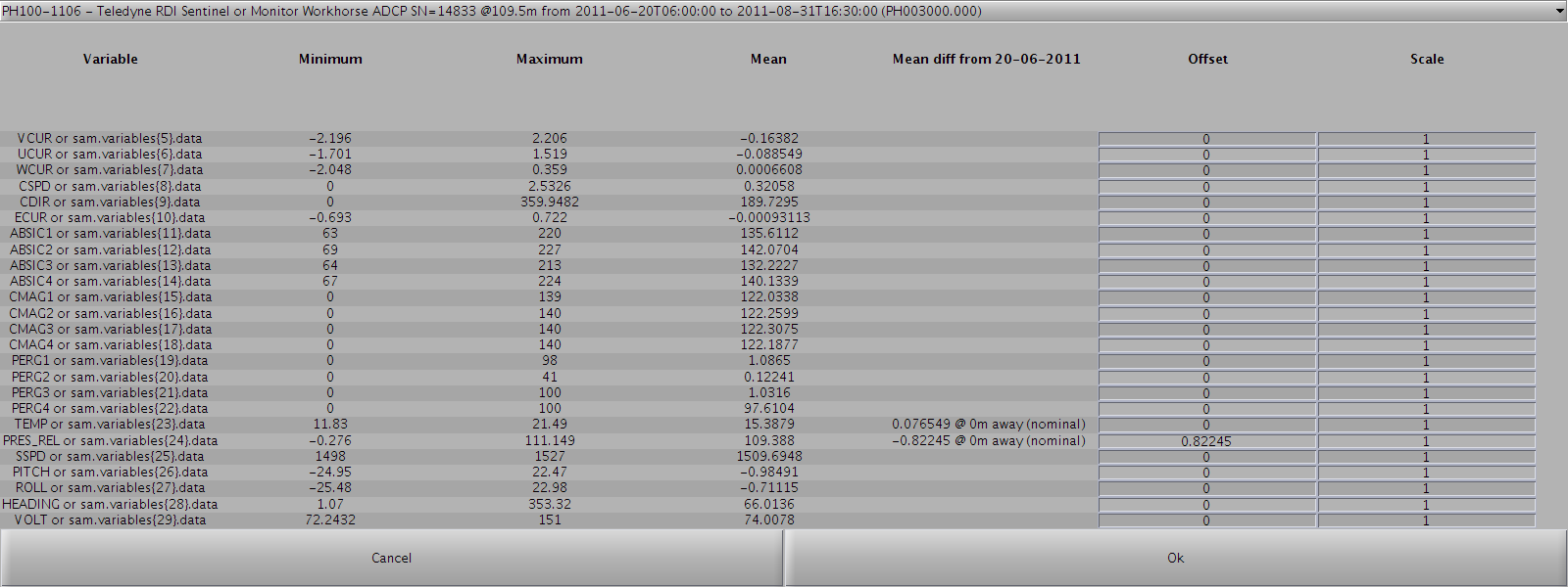
The GUI not only can take scalar values but also any Matlab statement, including the sam data structure representing the currently selected instrument.
The GUI shows for each parameter the minimum, maximum and mean value found for the current dataset. A mean difference with the nearest available sensor is shown when possible. If one would like to offset a parameter of the current instrument ibased on the mean difference with the nearest same sensor then the offset should be set such that:
offset = - mean diff
pressureRelPP adds a PRES_REL variable to the given data sets, if not already exist and if they contain a PRES variable.
PRES values are taken and an offset is applied to create PRES_REL values. Useful for instruments which pressure sensor is providing absolute pressure information, so that we can also have a relative pressure (usually to the surface) to be consistent with Seabird pressure sensor for example as they usually provide relative pressure.
A pressureRelPP.txt configuration file allows the user to define default offset values to be applied for identified instrument. See example below :
% Default pressure offset value used by pressureRelPP adding it to PRES variable
% to create PRES_REL variable.
%
% In order to be able to apply different offsets for different sensors,
% the considered offsets is the one in front of the matching 'source'
% global atribute value. If no relevant 'source', use default.
%
% Each line is of the format:
%
%   source = offset
%

default = -10.1325
mySpecificInstrument = -10.13
Here, the default value -10.1325 is the actual value applied by Seabird on all their pressure sensor before outputting data in ASCII file format (.cnv).
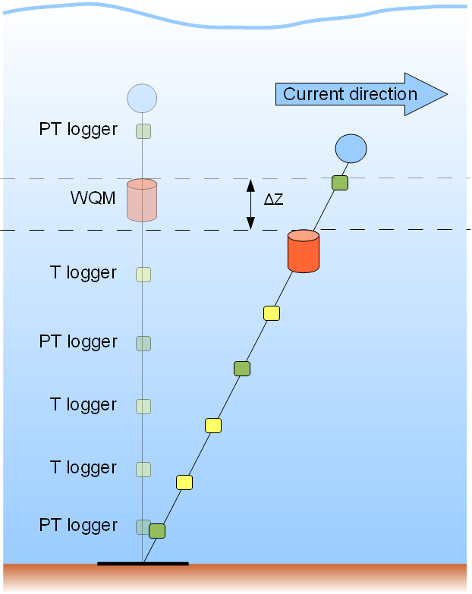
depthPP adds a DEPTH variable to the given data set, if not already exist. Useful as during strong current event, an instrument on a mooring is not likely to stay at its nominal depth but may record data at lower depth as the mooring is laying down.
This function uses the Gibbs-SeaWater toolbox (TEOS-10) to derive depth data from pressure and latitude.
When a data set is loaded without using a deployment database, DEPTH will be calculated from PRES or PRES_REL variables present in the dataset. Without any latitude metadata information, 1 dbar ~= 1 m is assumed. If latitude metadata information is documented then DEPTH will be updated taking this new information into account using the Gibbs-SeaWater toolbox.
When a data set is loaded using a deployment database, DEPTH will be calculated from PRES or PRES_REL variables present in the current instrument dataset or in the ones from the nearest pressure sensor on the mooring (1 or 2 nearest pressure sensors - 1 above and 1 below - are used when possible). Latitude metadata information si taken into account using the Gibbs-SeaWater toolbox. If latitude metadata information is updated then DEPTH will be updated taking this new information into account.
When an instrument data set doesn't contain any pressure/depth information, then the nearest pressure sensor (1 or 2 when possible) data on the mooring is considered and depth for the current instrument is linearly interpolated knowing the geometry/design of the mooring. Indeed, either global attributes instrument_nominal_height or instrument_nominal_depth must be documented for each instrument so that this routine can be performed properly.
A depthPP.txt configuration file allows the user to define which pressure sensor can be taken into account in order to compute the depth of an instrument that wouldn't have any pressure measurement. See example below :
% This file specifies how Depth should be computed when an instrument on a
% mooring doesn't have any pressure sensor. It enables the user to restrict
% the other instruments in the mooring with pressure information to be
% considered when calculating Depth for another without pressure information.
% It is used by the depthPP.m function.
%
% Each line is of the format:
%
%   option,     value
%
% where option can be used as follow :
%
% -same_family : Values can be yes or no. If value is yes, then only data
% sets with strings in their global attribute 'instrument' having something
% in common will be considered. Ex. : In a mooring equiped with an ADCP, a
% WQM, Aqualoggers 520PT and Aqualoggers 520T, the depth of the Aqualoggers
% 520T will be computed taking into account Aqualoggers 520PT pressure data
% only.
%
% -include : list of space delimited strings to be compared with data sets
% global attribute 'instrument'. If it has anything in common, this data
% set will be considered in the Depth computation.
% Ex. : include,        Aqualoggers
%
% -exclude : list of space delimited strings to be compared with data sets
% global attribute 'instrument'. If it has anything in common, this data
% set will not be considered in the Depth computation.
% Ex. : exclude,        ADCP WQM

same_family,   no
include,
exclude,       ADCP
In the case above, for any instrument without pressure measurements, any neighbouring instrument equipped with a pressure sensor (not necessarily same family) that is not an ADCP (their pressure sensor can be of poor quality) can be considered.
The algorithm selects the nearest neighbours and displays the default choices in the window below:
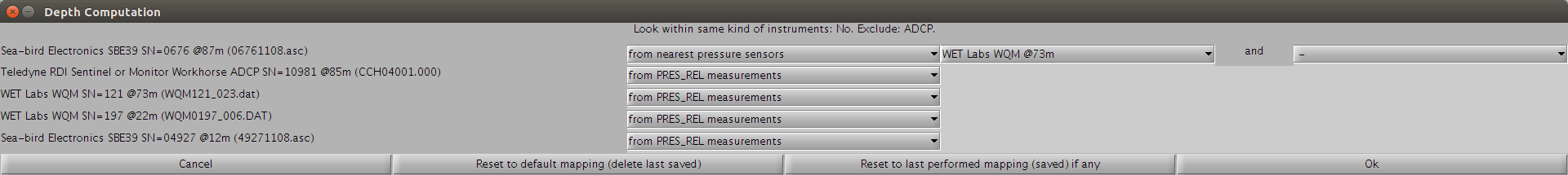
We can see that the first line within the window reflects our choices in depthPP.txt (any family, but no ADCP). Most of the instruments have pressure measurements from which DEPTH will be computed, except for the first one. Unfortunatelly for this one, we have only one nearest pressure sensor (no need to take into accound the second one in this case since it is lying above the instrument too).
If we were to change the content of depthPP.txt and wanted the window to reflect this, we would have to click on the button "Reset to default mapping (delete last saved)".
We can update the nearest neighbours that should be taken into account:
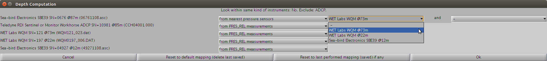
Or update the method used from which DEPTH will be computed:
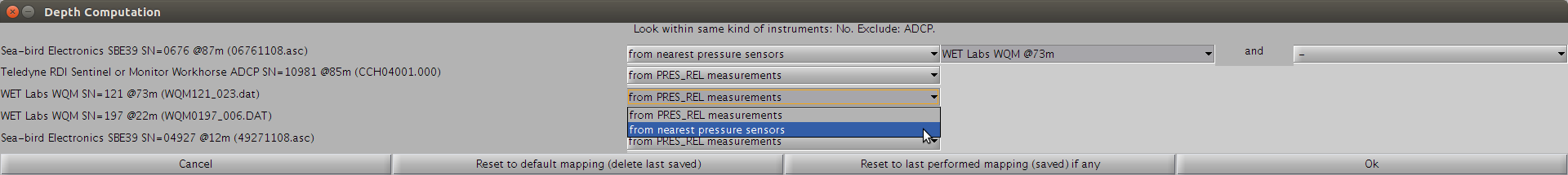
To get back to the last saved/performed mapping of methods and neighbours, just click on the button "Reset to last performed mapping (saved) if any".
salinityPP adds a salinity variable to the given data sets, if they contain conductivity, temperature and pressure/depth/nominal depth variables.
This function uses the Gibbs-SeaWater toolbox (TEOS-10) to derive salinity data from conductivity, temperature and pressure/depth/nominal depth. It adds the salinity data as a new variable in the data sets. Data sets which do not contain conductivity, temperature and pressure/depth/nominal depth variables or which already contain a salinity variable are left unmodified.
oxygenPP adds consistent oxygen variables to the given data sets. Whatever the original oxygen measurement is, new oxygen saturation variable (DOXS), oxygen solubility at atmospheric pressure variable (OXSOL_SURFACE), and finally oxygen variables expressed in umol/l (DOX1) and umol/kg (DOX2) will be added when possible.
This function uses the Gibbs-SeaWater toolbox (TEOS-10) to derive consistent oxygen data when possible from salinity, temperature and pressure. It adds oxygen data as new variables in the data sets. Data sets which do not contain oxygen, temperature, pressure and depth variables or nominal depth information are left unmodified.
From Argo document http://doi.org/10.13155/39795:
Oxygen data unit provided by Argo is umol/kg but the oxygen measurements are sent from Argo floats in another unit such as umol/L for the Optode and ml/L for the SBE-IDO. Thus the unit conversion is carried out by DACs as follows: O2 [umol/L] = 44.6596 . O2 [ml/L] O2 [umol/kg] = O2 [umol/L] / pdens Here, pdens is the potential density of water [kg/L] at zero pressure and at the potential temperature (e.g., 1.0269 kg/L; e.g., UNESCO, 1983). The value of 44.6596 is derived from the molar volume of the oxygen gas, 22.3916 L/mole, at standard temperature and pressure (0 C, 1 atmosphere; e.g., Garcia and Gordon, 1992). This unit conversion follows the "Recommendations on the conversion between oxygen quantities for Bio-Argo floats and other autonomous sensor platforms" by SCOR Working Group 142 on "Quality Control Procedures for Oxygen and Other Biogeochemical Sensors on Floats and Gliders" [RD13]. The unit conversion should always be done with the best available temperature, i.e., the one of the CTD unit.
soakStatusPP adds distinct diagnostic variables for tempreature, conductivity and dissolved oxygen which will help assessing the quality of the surface soak performed before the CTD was lowered. The depth, elapsed time and conductivity frequency are used to infer when the actual surface soak starts and diagnostic variables are created based on the elapsed time. This pre-processing routine is especially useful in conjunction with the CTDDepthBinPP pre-processing routine and the CTDSurfaceSoakQC test for CTD casts that might have not respected a minimum 3min surface soak (most of the early casts in South Australia for example).
This pre-processing routine is for use in profile mode only with .cnv files that haven't been vertically binned by SeaBird software. Indeed, vertically binned files don't have an elapsed time information anymore.
Diagnostic variables have 4-level values:
- -1: No Soak Status determined (usually elapsed time missing).
- 0: Pump Off and/or Minimum Soak Interval has not passed - data from sensor supplied by pump.
- 1: Pump On and first Minimum Soak Interval has passed - data from sensor are probably OK.
- 2: Pump On and Optimal Soak Interval has passed - data from sensor assumed to be good.
The following default minimum and optimal soak time values for each parameter can be modified by editing the soakStatusPP.txt:
| Parameter | Minimum soak time in sec | Optimal soak time in sec |
|---|---|---|
| Temperature | 60 | 70 |
| Conductivity | 70 | 90 |
| Oxygen | 150 | 180 |
CTDDepthBinPP averages the data which lies on vertical bins of size 1m (default value configurable via the CTDDepthBinPP.txt file). Only data with previous surface soak diagnostic variables of values >= 1 and SBE flag 'good' are considered during the averaging process. Diagnostic variables are also binned by considering the worst value in the bin.
This routine adds disolved oxygen variables DOXS, DOXY_TEMP and DOX1 to the given dataset if they contain pressure/depth information and analog voltages from Rinko temperature and DO sensors. It uses the RINKO III Correction method on Temperature and Pressure with instrument and calibration coefficients as well as atmospheric pressure at the time of calibration. These instrument and coefficients calibaration should be documented in rinkoDoPP.txt.
This routine transforms Aquatracka analog output into SI units for the following parameters CHLF, TURBF, CHR and CHC. It uses the following formula:
PARAM = scale_factor*10^(PARAM_analog) + offset
Variables scale_factor and offset are taken from calibration sheets and should be documented in aquatrackaPP.txt.
transformPP prompts the user to select from a list of transformation functions for the variables in the given data sets.
A transformation function is simply a function which performs some arbitrary transformation on a given data set.
A transformPP.txt configuration file allows the user to define which variable is to be applied which transformation. See example below :
% Default transformations for different variables. Each entry is of the form:
%
%   variable_name = transform_name
%
% If a variable is not listed, the default is no transformation.
%

DOXRAW = sbe43OxygenTransform
The following variable transformation is available in the toolbox:
sbe43OxygenTransform is an implementation of SBE43 oxygen voltage to concentration data transformation, specified in Seabird Application Note 64:
In order to derive oxygen, the provided data set must contain TEMP, PRES and PSAL variables.
magneticDeclinationPP computes a theoretical magnetic declination, for any data set relying on a magnetic compass, using NOAA's Geomag v7.0 software and the IGRF12 model. A different version of IGRF can be used if the relevant .COF file is in Geomag directory and the geomag.txt entry 'model' is documented properly. The actual location of the mooring, the instrument nominal depth (if deeper than 1000m, 1000m depth is considereed instead) and the date in the middle of the time_coverage_start and time_coverage_end of the dataset (it is assumed that the declination variation which occurs during the deployment time period is negligeable compared to the angular resolution of the data) are given as inputs for Geomag when using a deployment database. When not using any deployment database, a window prompts the user for this information. This computed magnetic declination is documented in a global attribute and a correction from it is applied to any data relying on a magnetic compass when it still refers to magnetic North so that it finally refers to true North.
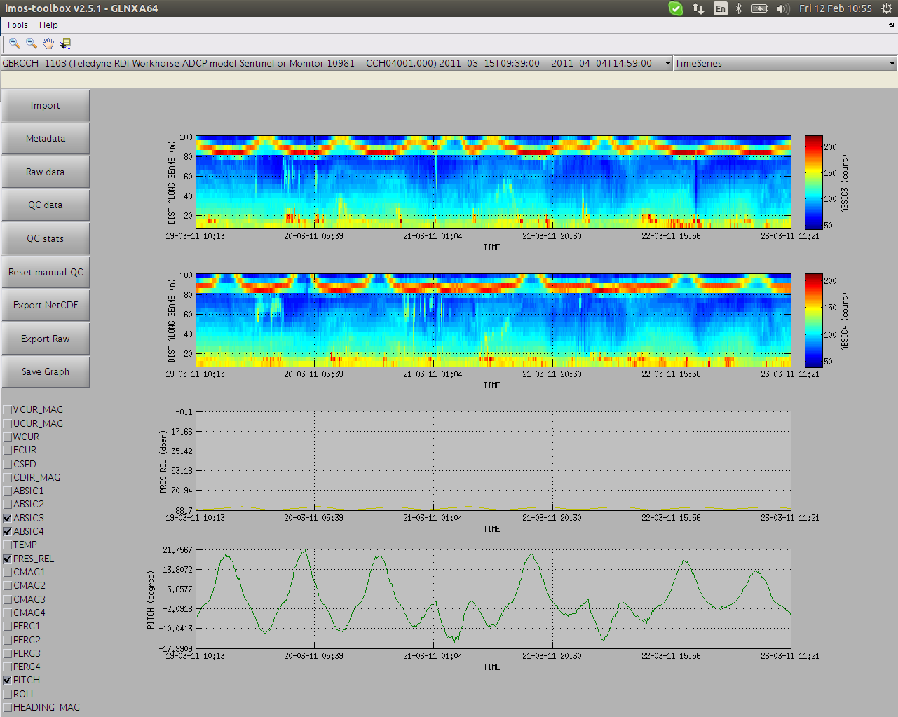
This routine derives acoustic backscatter intensity values in dB from values in counts by multiplying by a coeficient that can be set in absiDecibelBasicPP.txt (default value is 0.45).
See this discussion on Nortek's forum and this document.
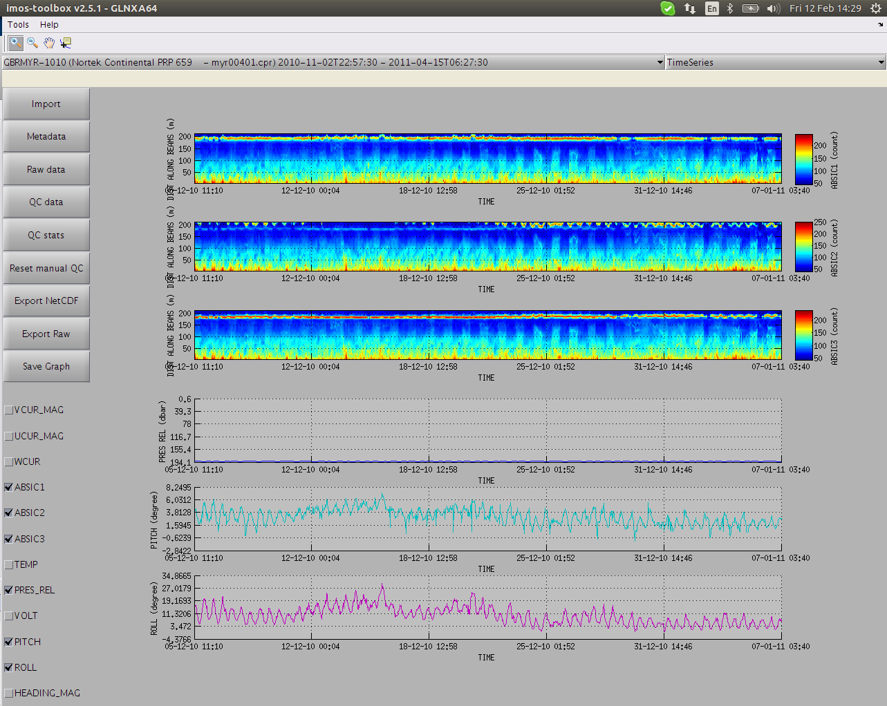
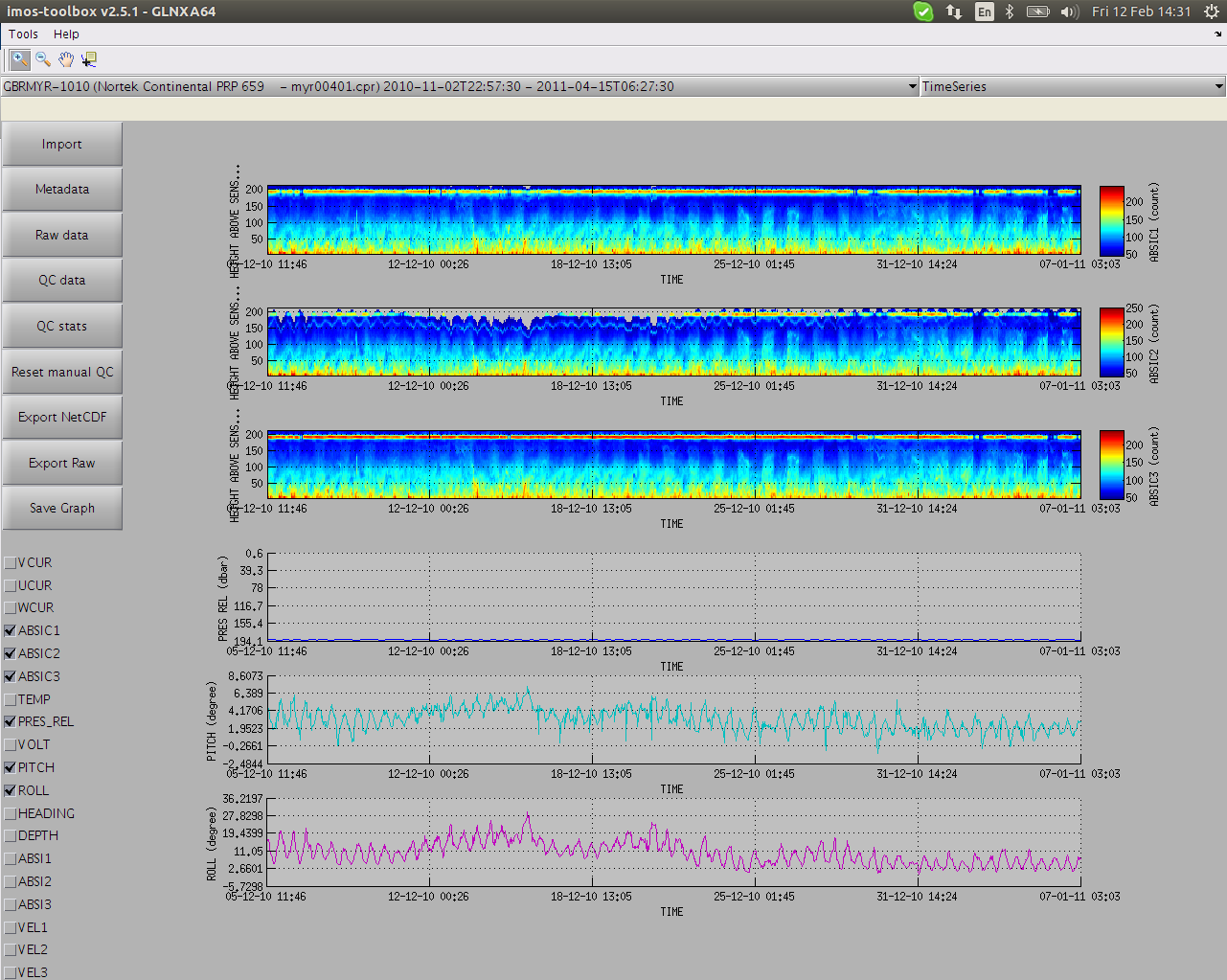
This routine performs a vertical bin-mapping (tilt correction) on any supported RDI or Nortek adcp (except Signature) variable expressed in beams coordinates and which is function of DIST_ALONG_BEAMS into a HEIGHT_ABOVE_SENSOR dimension if the velocity data found in this dataset is already a function of HEIGHT_ABOVE_SENSOR or if there is some velocity data in beam coordinates.
For every beam, each bin has its vertical height above sensor inferred from the tilt information. Data values are then interpolated at the nominal vertical bin heights (which is when tilt is 0).
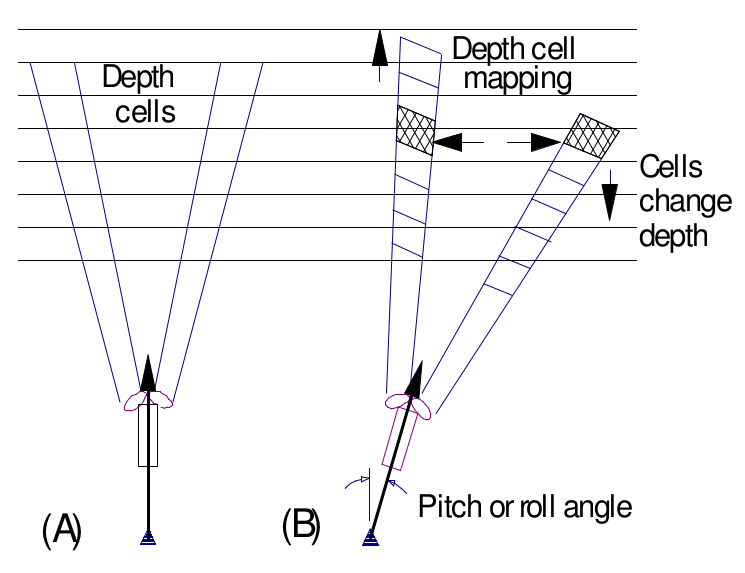
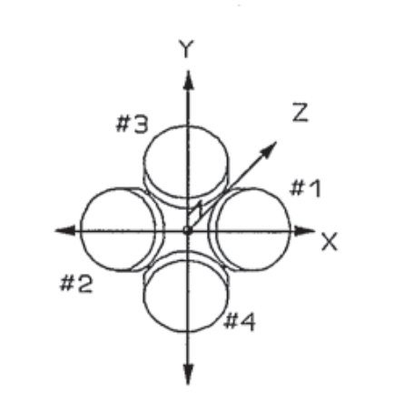
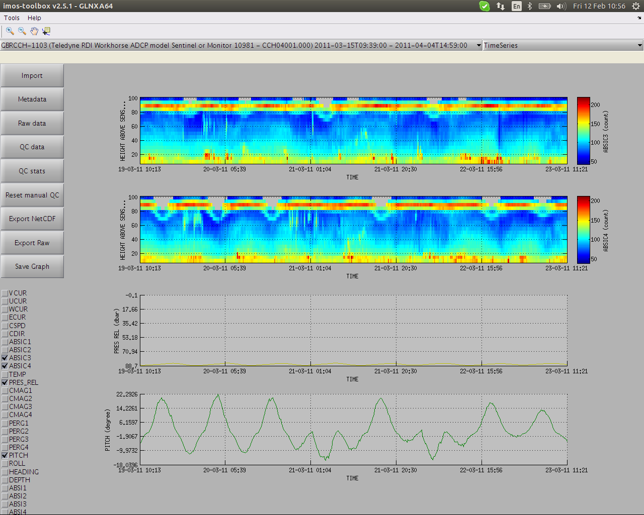
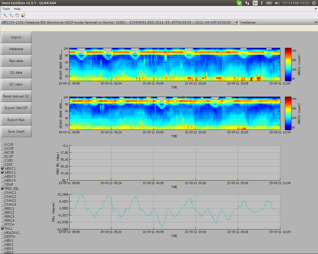
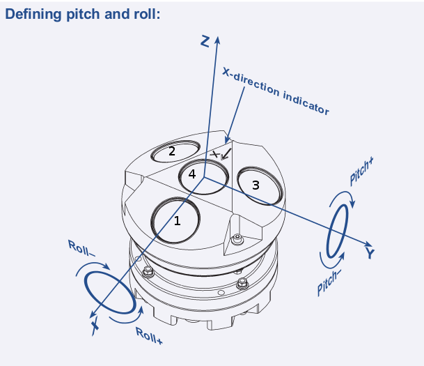
For RDI 4 beams ADCPs it is assumed that the beams are in a convex configuration such as beam 1 and 2 (respectively 3 and 4) are aligned on the pitch (respectively roll) axis. For an upward looking ADCP, when pitch is positive beam 3 is closer to the surface while beam 4 gets further away. When roll is positive beam 2 is closer to the surface while beam 1 gets further away.
Pitch impact on beams 3 and 4:
 Pitch corrected:
Roll impact on beams 1 and 2:
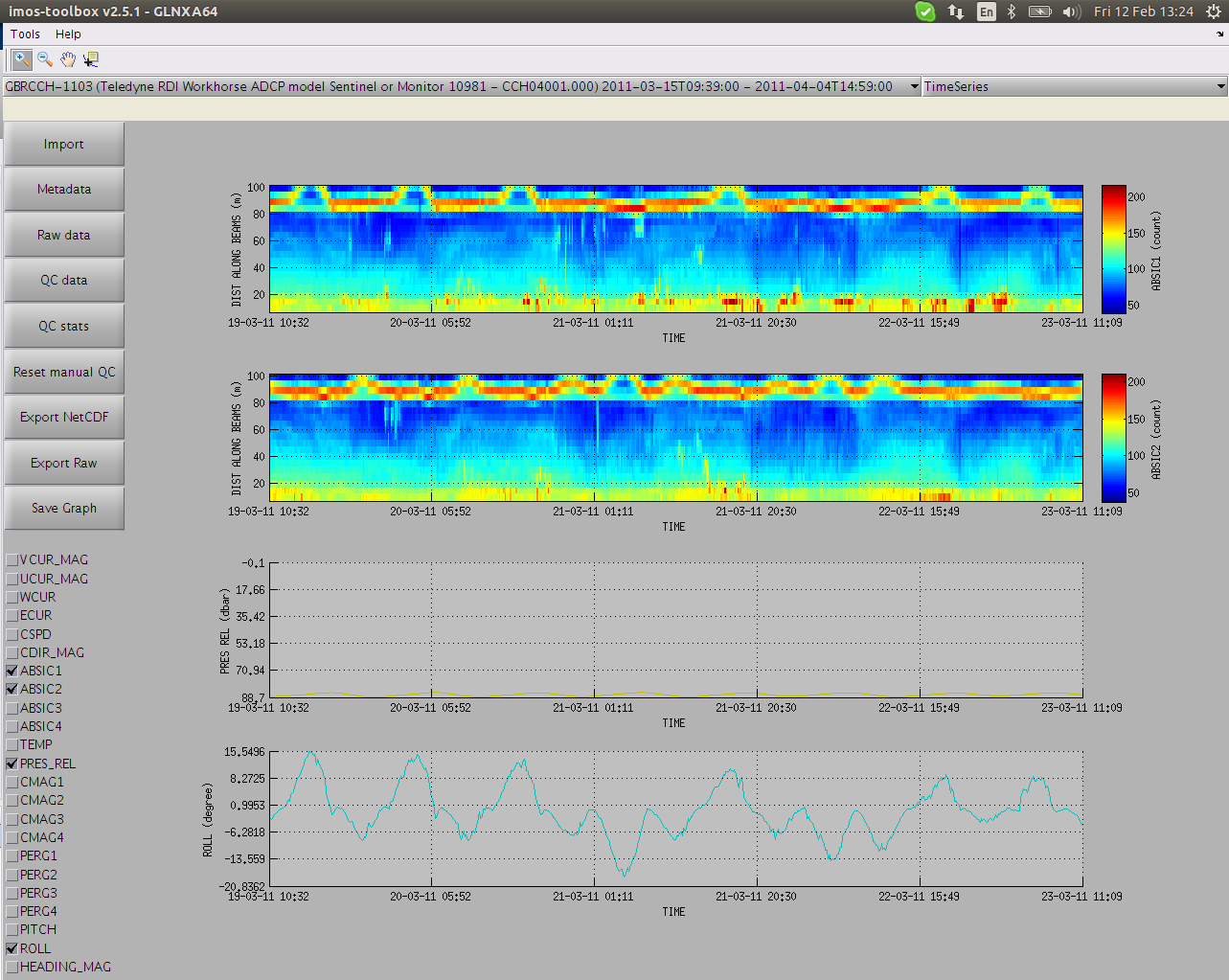 Roll corrected:
For Nortek 3 beams ADCPs, it is assumed that the beams are in a convex configuration such as beam 1 and the centre of the ADCP are aligned on the roll axis. Beams 2 and 3 are symetrical against the roll axis. Each beam is 120deg apart from each other. For an upward looking ADCP, when pitch is positive beam 1 is closer to the surface while beams 2 and 3 get further away. When roll is positive beam 3 is closer to the surface while beam 2 gets further away.
Pitch and roll impact on all beams:
 Pitch and roll corrected:
In combination with adcpNortekVelocityEnu2BeamPP and adcpNortekVelocityBeam2EnuPP, it is possible to perform bin-mapping on Nortek velocity data comparatively as with Nortek Storm software:
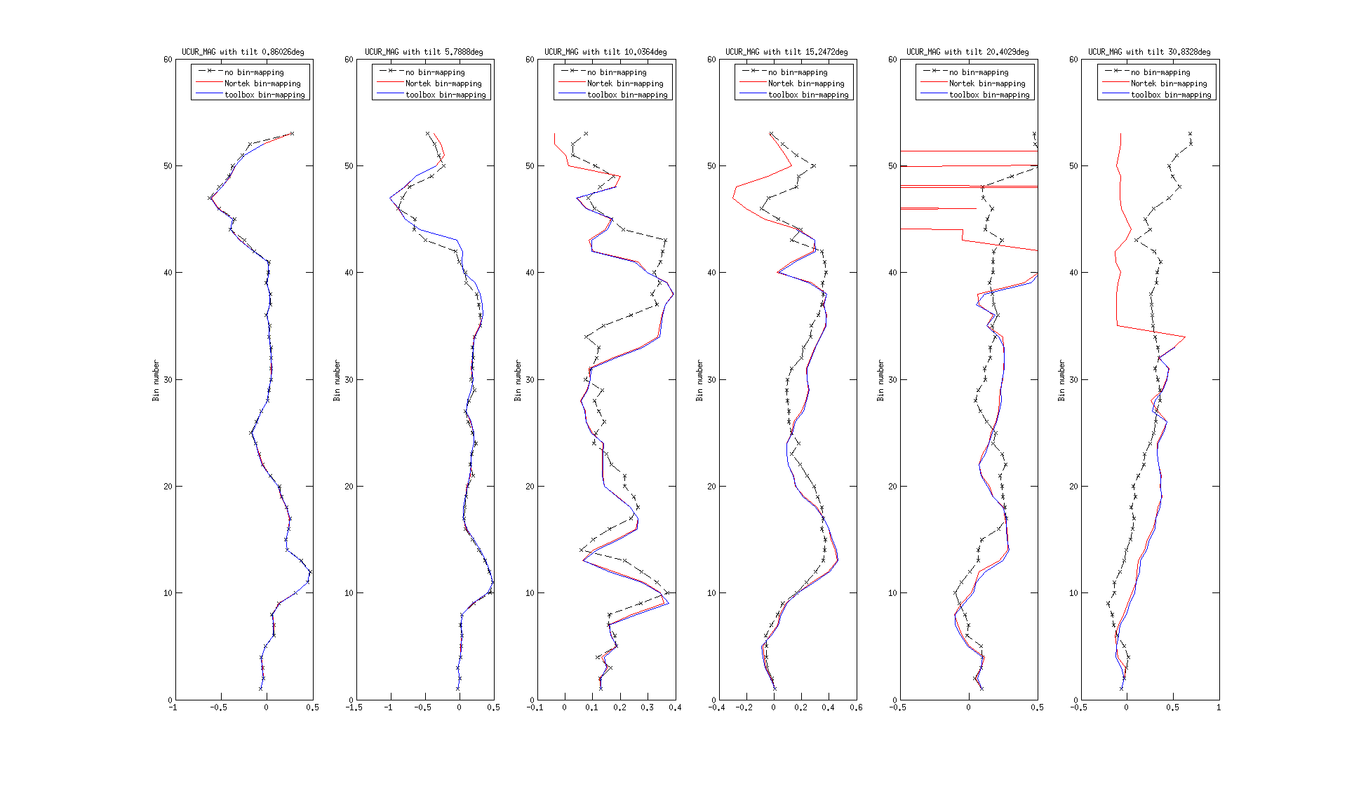
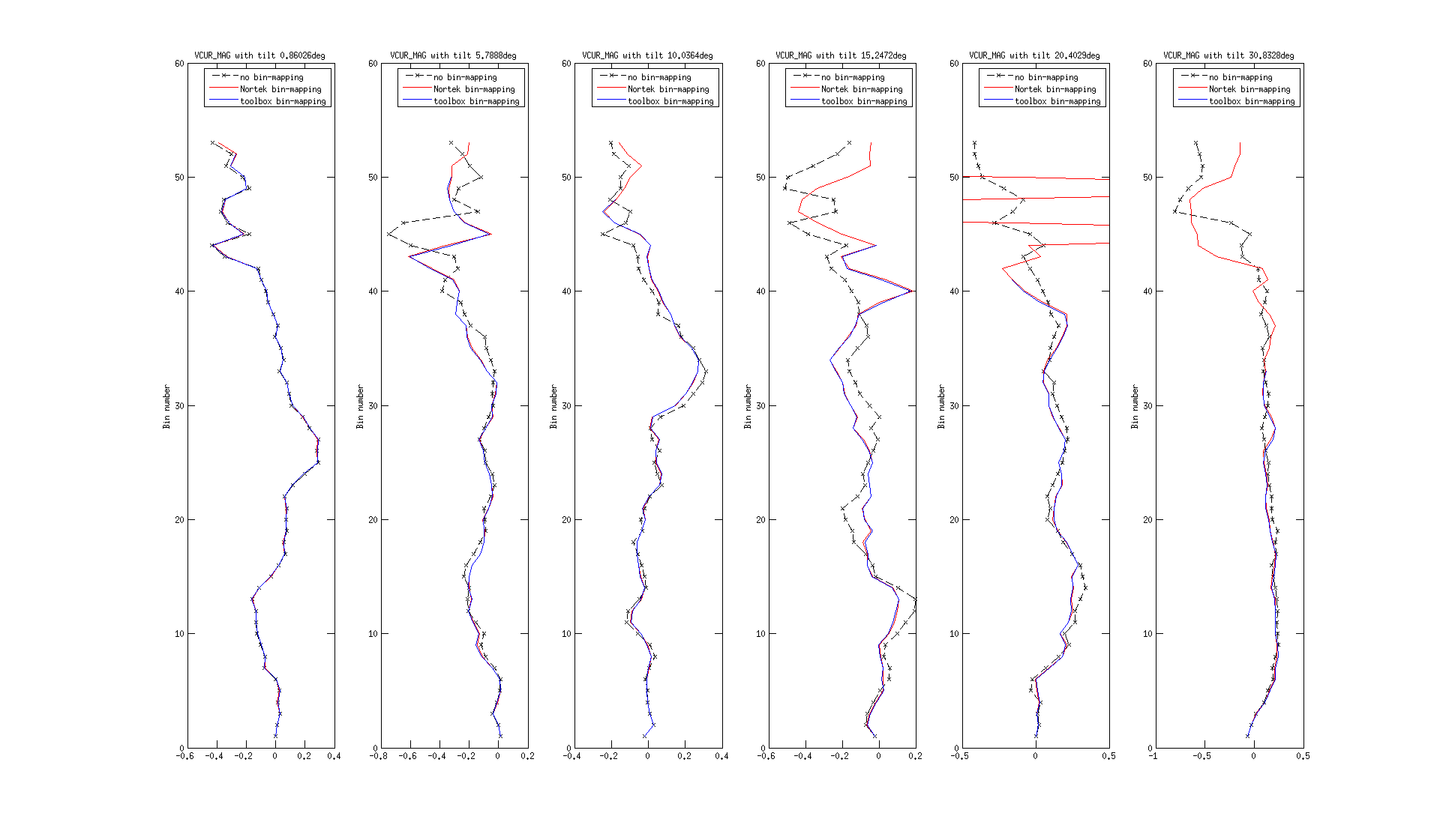
With increasing tilts, one of the ADCP beam is looking more and more horizontally through the water. Because the range is limited, then we will have less and less chance to 3 beams available for bin-mapping on the vertical axis (see bin-mapping above), hence we loose range on the vertical axis. The bin mapping performed by Nortek doesn't display such a behaviour and looks suspect for the furthest bins during important tilt.
Coordinate transformation from ENU to Beam of Nortek ADCP velocity data - adcpNortekVelocityEnu2BeamPP
This routine transforms Nortek velocity data (except for Signature ADCPs) expressed in Easting Northing Up (ENU) coordinates to Beam coordinates. Parameters VEL1, VEL2 and VEL3 are added to the FV01 dataset. Following Nortek's documentation on coordinate transforms, we remove the ADCP attitude information (upward/downward looking, heading, pitch and roll) and then apply the provided XYZ to Beam matrix transformation.
Coordinate transformation from Beam to ENU of Nortek ADCP velocity data - adcpNortekVelocityBeam2EnuPP
This routine transforms Nortek velocity data (except for Signature ADCPs) expressed in Beam coordinates to Easting Northing Up (ENU) coordinates. Parameters UCUR, VCUR and WCUR are updated in the FV01 dataset. Following Nortek's documentation on coordinate transforms, we apply the provided Beam to XYZ matrix transformation to which we add the ADCP attitude information (upward/downward looking, heading, pitch and roll).
Coordinate transformation from Beam to ENU of Teledyne ADCP velocity data - adcpWorkhorseVelocityBeam2EnuPP
This routine transforms Teledyne velocity data (workhorse ADCPs) expressed in Beam coordinates to Easting Northing Up (ENU) coordinates. The parameters VEL1, VEL2, VEL3, VEL4 are transformed to UCUR, VCUR, WCUR and ECUR using the ADCP attitude information (upward/downward looking, heading, pitch and roll) and the respective rotation matrices. The transformed parameters are only available in the FV01 dataset (i.e., after executing/triggering the Quality Control button in the main window).
The transformation follows standard procedures from the [teledyne coordinate manual] document. In short, the instrument beam coordinates are rotated to Earth coordinates with the following fields:
VEL_ENU(T,N) = H(T) * GP(T) * AR(T) * I * BEAM_VEL(T), ∀ T.
Where H is the heading matrix, GP is the Gimbal Pitch matrix, and AR the Adjusted Roll matrix. These matrices are all bin-invariant, whereas I is a constant Beam to Instrument Matrix associated with the respective ADCP model (beam angle, physical beam layout). The BEAM_VEL is the velocity beam matrix (time/bin dependent) and is composed of the four beam components dimensions as columns, while individual values at each bin along the rows. The computation is done via iteration along time (T):
for t in each T:
VEL_ENU[4,N] = ( H[4x4] x GP[4x4] x AR[4x4] x I[4,4] ) x BEAM_VEL[4,N].
end
Where x denotes matrix multiplication and the final matrix is in the East, North, Up, and Neutral/Error velocity components.
For meaningful conversions from beam to ENU (both Workhorses and Norteks), the recommended order of PP routines is:
... → binMappingPP → adcpWorkhorseVelocityBeam2EnuPP/adcpNortekVelocityBeam2EnuPP → magneticDeclinationPP → ...
This routine generates polar velocity variables (CSPD, CDIR) from cartesian components corrected for magnetic declination (UCUR, VCUR). It is recommended that this routine is called at the bottom of the PP execution list. If the dataset is not corrected for magnetic declination - UCUR_MAG & VCUR_MAG are the only available variables - no polar components are created.
[teledyne coordinate manual] Teledyne RD Instruments (2008). ADCP Coordinate Transformation, Formulas and Calculations, Teledyne RD Instruments. P/N 951-6079-00 (January 2008).