-
Notifications
You must be signed in to change notification settings - Fork 32
3D Advecting Field Loop
This test illustrates the ability of a code to preserve cholla/builds/make.type.mhd). Full initial conditions can be found in cholla/src/grid/initial_conditions.cppunder Advecting_Field_Loop().
#
# Parameter File for an MHD Advecting Field Loop as defined in
# [Gardiner & Stone 2008](https://ui.adsabs.harvard.edu/abs/2008JCoPh.227.4123G/abstract)
#

################################################
# number of grid cells in the x dimension
nx=128
# number of grid cells in the y dimension
ny=128
# number of grid cells in the z dimension
nz=256
# final output time
tout=2.0
# time interval for output
outstep=2.0
# name of initial conditions
init=Advecting_Field_Loop
# domain properties
xmin=-0.5
ymin=-0.5
zmin=-1.0
xlen=1.0
ylen=1.0
zlen=2.0
# type of boundary conditions
xl_bcnd=1
xu_bcnd=1
yl_bcnd=1
yu_bcnd=1
zl_bcnd=1
zu_bcnd=1
# path to output directory
outdir=./

#################################################
# Parameters for advecting field loop problem
# initial density
rho=1.0
# velocity in the x direction
vx=1.0
# velocity in the y direction
vy=1.0
# velocity in the z direction
vz=2.0
# initial pressure
P=1.0
# amplitude of the loop/magnetic field background value
A=0.001
# Radius of the Loop
radius=0.3

# value of gamma
gamma=1.666666666666667
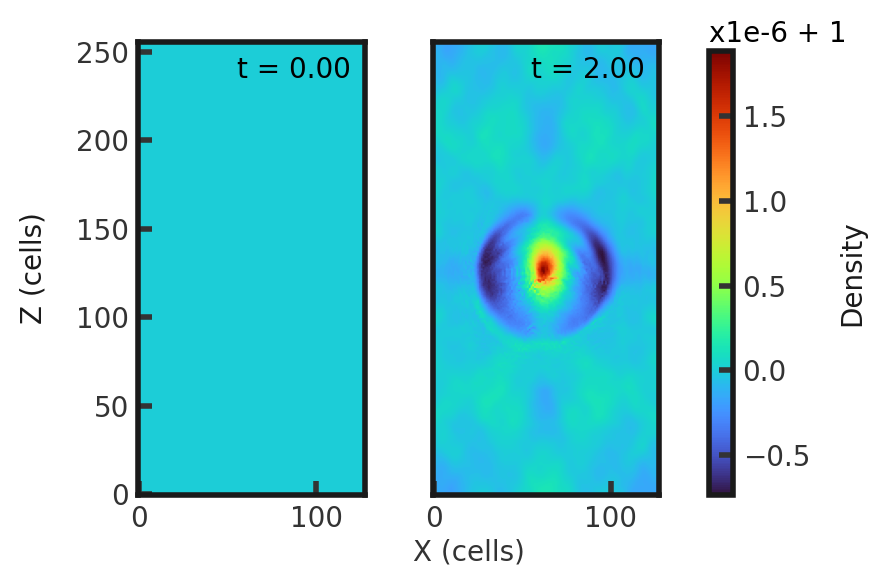
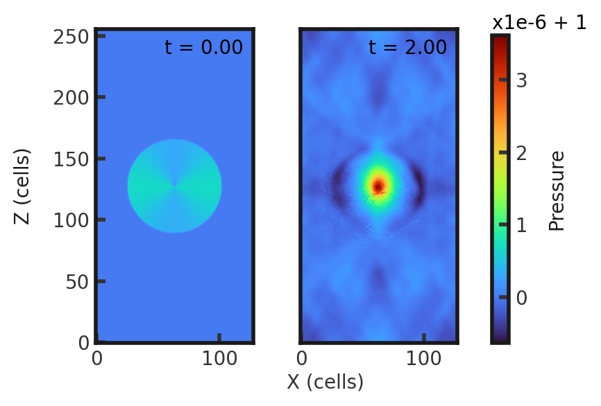
Upon completion, you should obtain 2 output files. The initial and final densities (in code units) of a slice along the y-midplane is shown below. Examples of how to plot projections and slices can be found in cholla/python_scripts/Projection_Slice_Tutorial.ipynb.


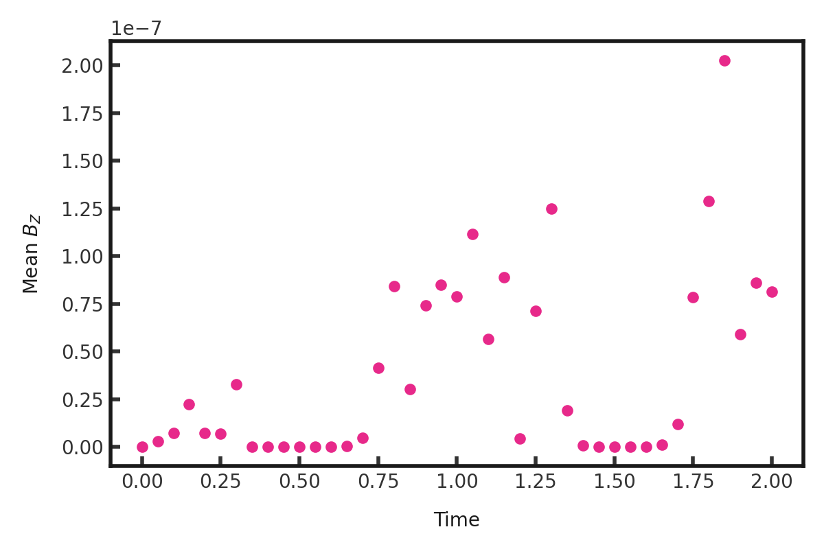
We can take a slice along the y-midplane of the z component of the magnetic field, averaging the value over the slice, at more frequent outputs to test how well the code preserves
 By changing the outstep to 0.05, you will obtain 41 output files and can obtain the below animation (10 fps):
advecting-field-loop-density.mp4
We see the loop moving to the upper right, prompting fluctuations in the background as it transitions out of view before returning in the lower left.